All your base R belong to us: small data and expansive analytics in base R
This rendering was constructed from an original PowerPoint presentation. Corrections of original text are indicated as “[corrected: X]”, redactions as “[redacted: X]”, and names withheld as “[generalized: X]”. Handouts and other auxiliary sources mentioned in the presentations are not available. The content of each presentation was believed to be correct and valid at the time of the presentation. This content, including references and links within the slides, has not been checked or updated when preparing this site. This rendering was facilitated by Anthropic Claude agentic tools for automated text extraction through computer vision and for assistance with compiling the completed sets.
Setting: All your base R belong to us: small data and expansive analytics in base R, 2019-10-24. CDC’s R Users Group.
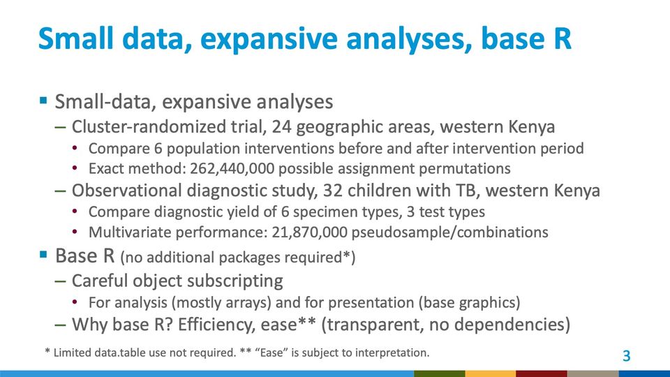
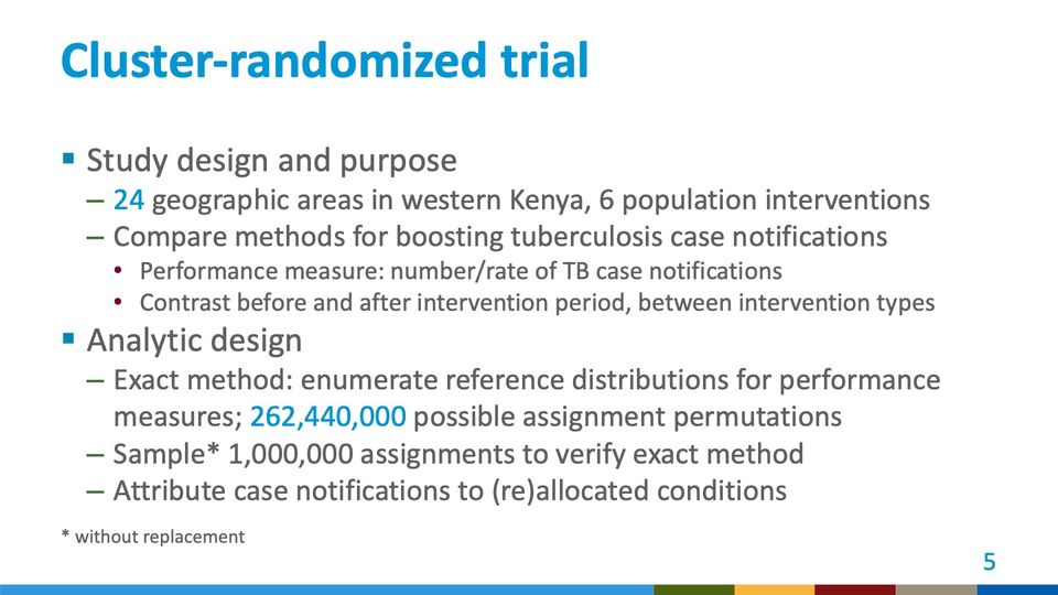
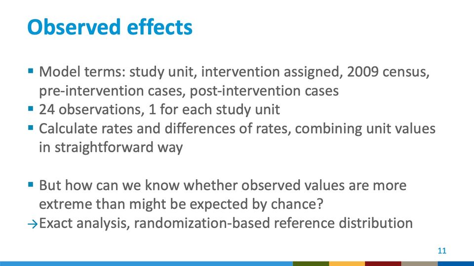
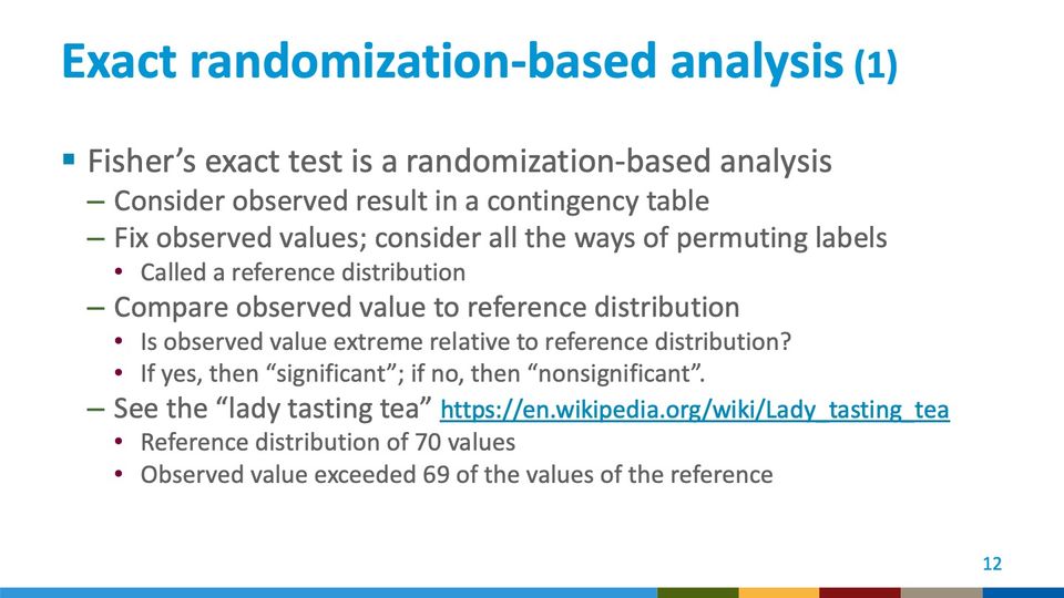
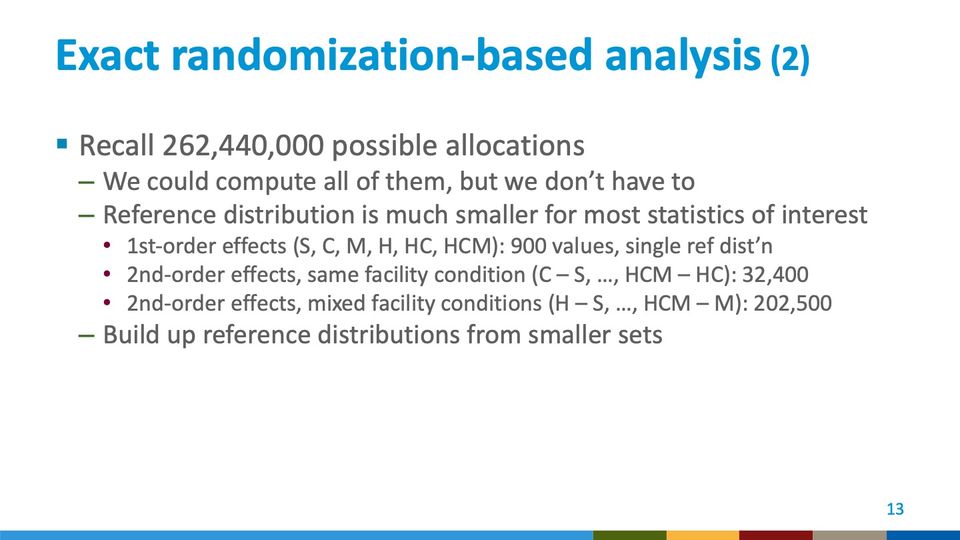
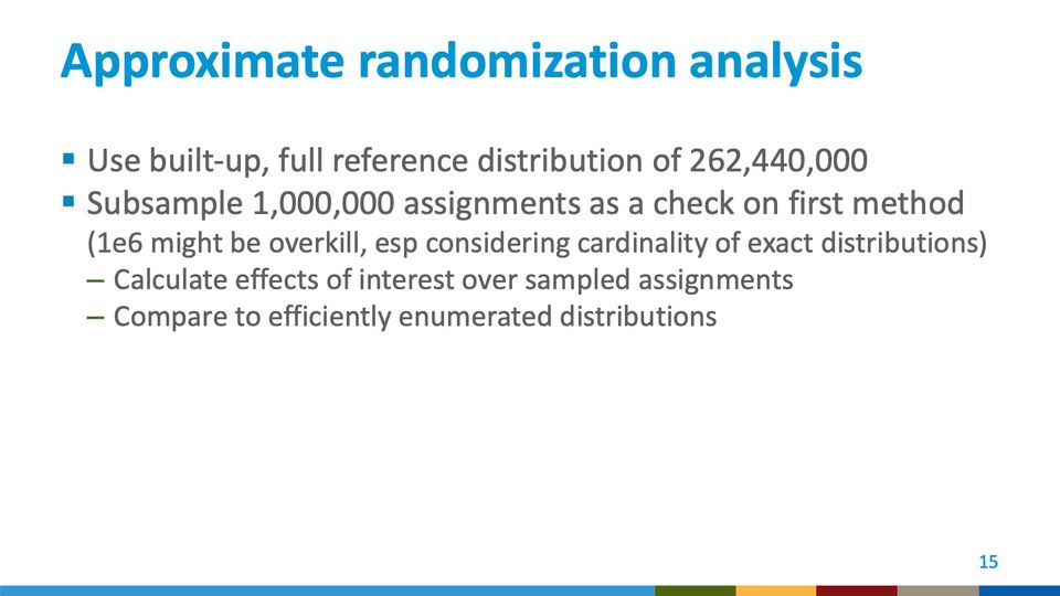
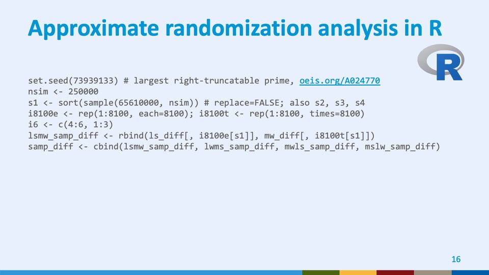
This presentation set up expansive analysis of 2 small datasets from studies in western Kenya. In a cluster-randomized trial, we allocated 6 population-level interventions to 24 geographic areas and compared findings before and after an intervention period. The exact method from these small numbers worked from 262,440,000 possible assignment permutations. In an observational diagnostic study of 32 children with laboratory evidence of tuberculosis (TB), we drew 10,000 pseudosamples of 729 specimen combinations to approximate the multivariate performance of 21,870,000 pseudosample combinations. I performed the entire analysis in base R using careful subscripting. I could perhaps have used other packages, or these days Python, but at the time it was intellectually satisfying to work with efficiency, transparency, and a lack of library dependencies while exercising granular control.
Text in the picture
Center for Surveillance, Epidemiology, and Laboratory Services
Abbreviations: CDC = Centers for Disease Control and Prevention; HHS = Department of Health and Human Services.

Text in the picture
CATS: ALL YOUR BASE R BELONG
TO US.
Abbreviations: TB = tuberculosis.
Abbreviations: TB = tuberculosis.
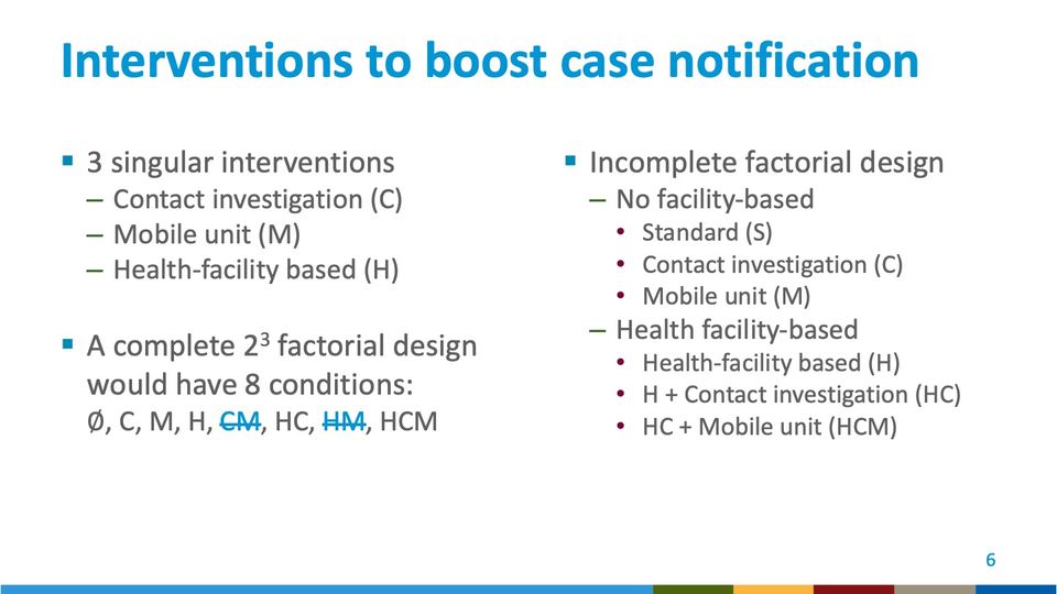
Abbreviations: HC = health-facility enhancement plus contact investigation (trial condition H + C); HCM = health-facility enhancement plus contact investigation plus mobile unit (trial condition H + C + M); HM = health-facility enhancement plus mobile unit (trial condition H + M).
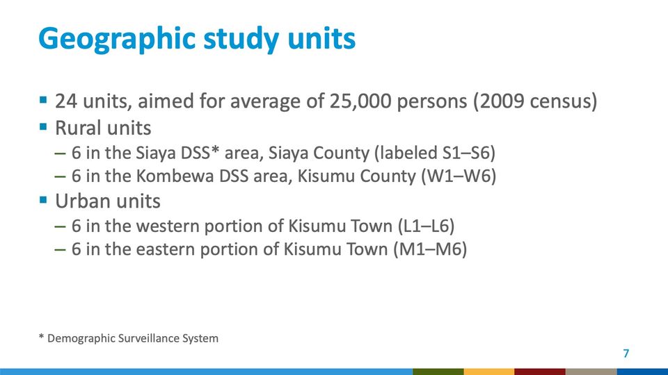
Abbreviations: DSS = demographic surveillance system.
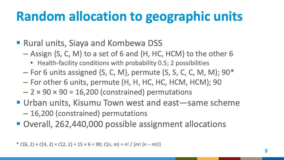
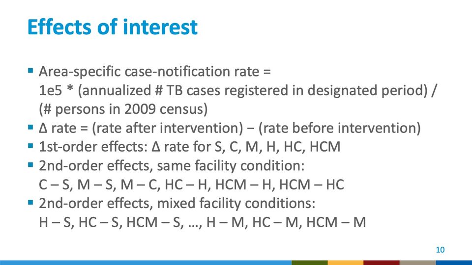
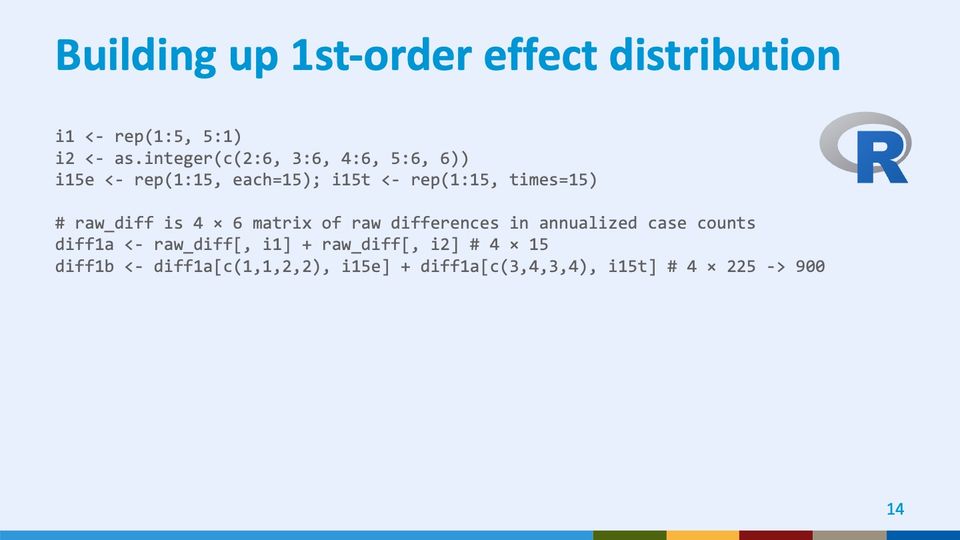
In the 6 units with enhanced health-facility conditions, there were 90 ways to assign 3 conditions in pairs: C(6, 2), or 15, ways to assign 1 pair among the 6 units; C(4, 2), or 6, ways to assign another pair among the remaining 4 units, and C(2, 2), or 1, way to assign the third pair among the remaining 2 units, giving C(6, 2) × C(4, 2) × C(2, 2) = 15 × 6 = 90. Similarly, in the remaining 6 rural units, there were 90 ways to assign 3 pairs of interventions that did not involve enhanced case-finding at health facilities. These numbers 2 × 90 × 90 yielded 16,200 possible assignments, each with equal probability. C(6, 2) is notation for the number of way to choose 2 GSUs a set of 6 GSUs, also known as a binomial coefficient.
In factorial notation, C(n, m) = n! / [m! (n − m)!].
Abbreviations: DSS = demographic surveillance system; GSUs = geographic study units; HC = health-facility enhancement plus contact investigation (trial condition H + C); HCM = health-facility enhancement plus contact investigation plus mobile unit (trial condition H + C + M).
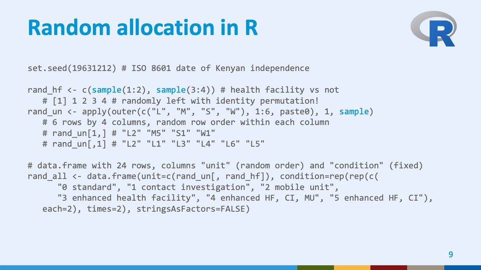
Abbreviations: CI = contact investigation; HF = health facility; ISO = International Organization for Standardization; MU = mobile unit.
Abbreviations: HC = health-facility enhancement plus contact investigation (trial condition H + C); HCM = health-facility enhancement plus contact investigation plus mobile unit (trial condition H + C + M); TB = tuberculosis.
Abbreviations: HC = health-facility enhancement plus contact investigation (trial condition H + C); HCM = health-facility enhancement plus contact investigation plus mobile unit (trial condition H + C + M).
- Panels
- 1
- Elements
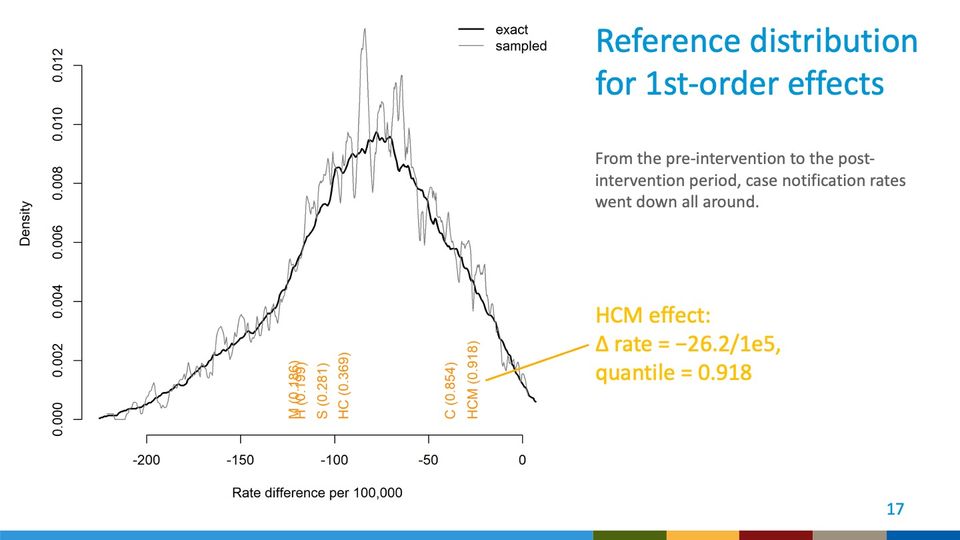
- 2 density curves (legend: exact, thick black line; sampled, thin gray line) depict density over rate difference; 6 rotated orange text labels stand just above the horizontal axis, each naming an effect with a value in parentheses; a yellow leader line runs from the HCM label to the callout text at right of the plot
- Horizontal
- Rate difference per 100,000; ticks from -200 to 0 in steps of 50; curves extend from about -225 to about 5, slightly beyond the outer ticks
- Vertical
- Density; ticks from 0.000 to 0.012 in steps of 0.002; the sampled curve's highest spike reaches about 0.013, just above the top tick
- Visible pattern
- Both curves rise from near zero at the far left, peak between about -85 and -70, and fall back to near zero at the right end, just past 0. The left tail is long and gradual, the right side shorter and steeper. The exact curve is fairly smooth and peaks near 0.0096; the sampled curve tracks it closely but is jagged throughout, with its largest swings near the peak. Four labels cluster between about -120 and -95, on the rising left side, and 2 stand apart on the falling right side, near -40 and -25.
Text in the picture
exact
sampled
M (0.186)
H (0.199)
S (0.281)
HC (0.369)
C (0.854)
HCM (0.918)
Abbreviations: HC = health-facility enhancement plus contact investigation (trial condition H + C); HCM = health-facility enhancement plus contact investigation plus mobile unit (trial condition H + C + M).
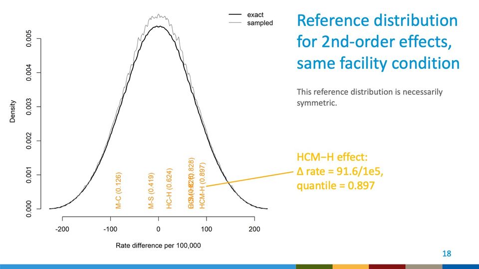
- Panels
- 1
- Elements
- 2 density curves (legend: exact, thick black line; sampled, thin gray line) depict density over rate difference; 6 rotated orange text labels stand just above the horizontal axis, each naming an effect with a value in parentheses, 2 of them overlapping; a yellow leader line runs from the HCM-H label to the callout text at right of the plot
- Horizontal
- Rate difference per 100,000; ticks from -200 to 200 in steps of 100; curves extend from about -225 to about 225, slightly beyond the outer ticks
- Vertical
- Density; ticks from 0.000 to 0.005 in steps of 0.001; curves peak at about 0.0054 (exact) and 0.0057 (sampled)
- Visible pattern
- Both curves are bell-shaped and symmetric about 0, rising from near zero at about -225 to a single peak at 0 and falling to near zero at about 225. They nearly coincide in the tails and shoulders; near the peak, from about -50 to 50, the sampled curve runs slightly above the exact one and is slightly ragged. One label on the left near -85 and one near -15; the other 4 bunch on the right between about 20 and 95, where 2 of them overlap.
Text in the picture
exact
sampled
M-C (0.126)
M-S (0.419)
HC-H (0.624)
[illegible]
HCM-H (0.897)
Abbreviations: HC = health-facility enhancement plus contact investigation (trial condition H + C); HCM = health-facility enhancement plus contact investigation plus mobile unit (trial condition H + C + M).
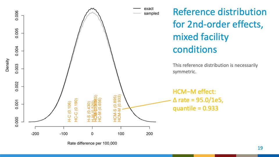
- Panels
- 1
- Elements
- 2 density curves (legend: exact, thick black line; sampled, thin gray line) depict density over rate difference; rotated orange text labels stand just above the horizontal axis, each naming an effect with a value in parentheses, several overlapping near the center; a yellow leader line runs from the HCM-M label to the callout text at right of the plot
- Horizontal
- Rate difference per 100,000; ticks from -200 to 200 in steps of 100; curves extend from about -220 to about 220, slightly beyond the outer ticks
- Vertical
- Density; ticks from 0.000 to 0.006 in steps of 0.001; curves peak at about 0.0064 (exact) and 0.0062 (sampled), just above the top tick
- Visible pattern
- Both curves are bell-shaped and mirror each other about 0, rising from near zero at about -220 to a single peak at 0 and falling to near zero at about 220. The exact curve runs slightly above the sampled one around the peak, from about -75 to 75, and the 2 nearly coincide in the tails. Two labels on the left near -85 and -60, a cluster of overlapping labels sits between about -15 and 25, and 2 labels on the right near 80 and 95.
Text in the picture
exact
sampled
H-C (0.106)
HC-C (0.190)
H-S (0.430)
[illegible]
HC-M (0.656)
HCM-S (0.895)
HCM-M (0.933)
Abbreviations: HC = health-facility enhancement plus contact investigation (trial condition H + C); HCM = health-facility enhancement plus contact investigation plus mobile unit (trial condition H + C + M).
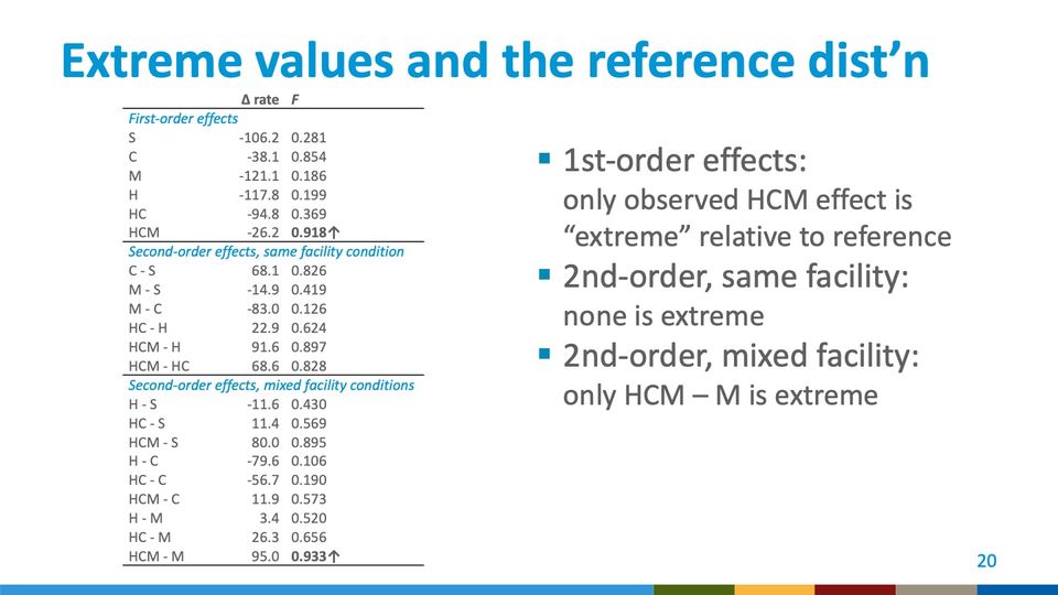
Abbreviations: HC = health-facility enhancement plus contact investigation (trial condition H + C); HCM = health-facility enhancement plus contact investigation plus mobile unit (trial condition H + C + M).
Abbreviations: TB = tuberculosis.
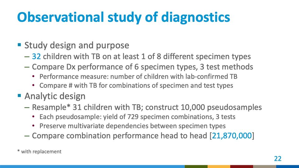
Abbreviations: Dx = diagnosis; TB = tuberculosis.
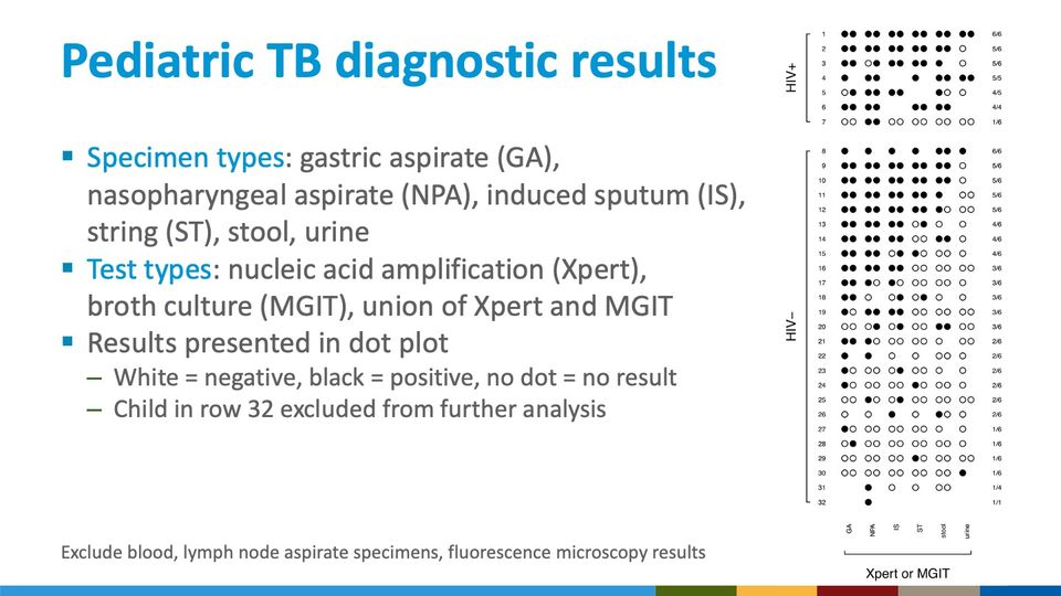
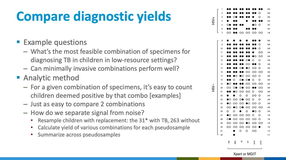
- Panels
- 1
- Elements
- Dot plot of 32 numbered rows by 6 specimen-type columns; each cell holds up to 2 circles, filled black or open white, or is empty; rows in 2 bracketed groups labeled HIV+ (rows 1 to 7) and HIV– (rows 8 to 32); a fraction label at the right end of each row, ranging from 6/6 to 1/1
- Horizontal
- 6 specimen-type columns, labeled vertically below as GA, NPA, IS, ST, stool, urine, bracketed together under the label Xpert or MGIT; up to 2 dots side by side per column
- Vertical
- 32 rows numbered 1 to 32 from top to bottom, with a gap between rows 7 and 8 separating the 2 HIV groups
- Visible pattern
- Within each HIV group the rows run from mostly black at the top to mostly white at the bottom, and the fraction labels at the right descend in step, from 6/6 near the top of each group to 1/6 near its bottom. Black dots are densest in the GA, NPA and IS columns; the ST, stool and urine columns are mostly white below the first several rows of each group. Some cells hold a single dot rather than a pair, and some are empty. The last 2 rows carry the fewest dots, the last only a single black dot, under NPA.
Abbreviations: GA = gastric aspirate; HIV = human immunodeficiency virus; HIV+ = HIV-positive; IS = induced sputum; MGIT = Mycobacteria Growth Indicator Tube (liquid culture system); NPA = nasopharyngeal aspirate; ST = string test (specimen collection method); TB = tuberculosis; Xpert = Xpert MTB/RIF (Cepheid GeneXpert cartridge nucleic acid amplification test for TB and rifampicin resistance).
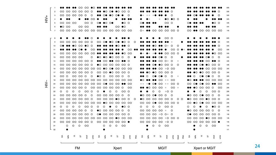
- Panels
- 1
- Elements
- Dot plot of 32 numbered rows by 27 test-and-specimen columns in 4 bracketed column groups; each cell holds up to 2 circles, filled black (positive), open white (negative), or small filled gray (contaminated or indeterminate), or is empty (no result); rows in 2 bracketed groups labeled HIV+ (rows 1 to 7) and HIV– (rows 8 to 32); a fraction label at the right end of each row, ranging from 6/6 to 1/1
- Horizontal
- 4 column groups, left to right: FM (GA, NPA, IS, ST, stool, urine); Xpert (GA, NPA, IS, ST, stool, urine, FNA); MGIT (GA, NPA, IS, ST, stool, urine, blood, FNA); Xpert or MGIT (GA, NPA, IS, ST, stool, urine); column labels set vertically below, group labels under brackets
- Vertical
- 32 rows numbered 1 to 32 from top to bottom, with a gap between rows 7 and 8 separating the 2 HIV groups
- Visible pattern
- The FM group is almost entirely white, with black dots in only a handful of rows, mostly near the top of each HIV group and in the last row. The Xpert and MGIT groups carry many more black dots, concentrated in the upper rows of each HIV group and in the GA, NPA and IS columns, thinning to mostly white toward the bottom. Small gray dots appear almost only in the MGIT group, scattered down many rows and most often in the stool column. The FNA and blood columns are sparse, with dots in only a few rows. The rightmost group, Xpert or MGIT, is the densest in black, and like the others runs from mostly black at the top of each HIV group to mostly white at the bottom; the fraction labels descend from 6/6 to 1/6 within each group.
Specimen types: gastric aspirate (GA), nasopharyngeal aspirate (NPA), induced sputum (IS), string (ST), stool, urine, blood, lymph node aspirate (FNA)
Test types: fluorescence microscopy (FM), nucleic acid amplification (Xpert), broth culture (MGIT), union of Xpert and MGIT
Abbreviations: FM = fluorescence microscopy; FNA = fine-needle aspirate (of a lymph node); GA = gastric aspirate; HIV = human immunodeficiency virus; HIV+ = HIV-positive; IS = induced sputum; MGIT = Mycobacteria Growth Indicator Tube (liquid culture system); NPA = nasopharyngeal aspirate; ST = string test (specimen collection method); TB = tuberculosis; Xpert = Xpert MTB/RIF (Cepheid GeneXpert cartridge nucleic acid amplification test for TB and rifampicin resistance).
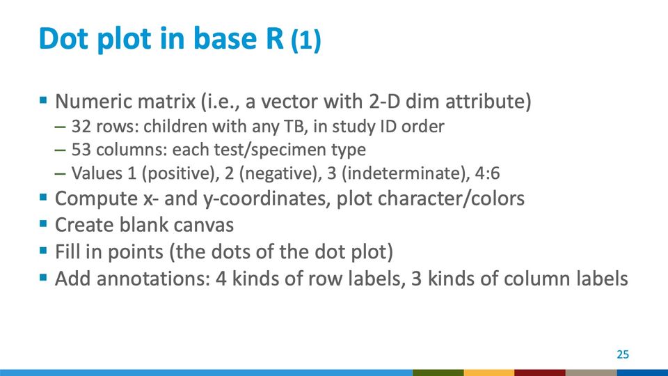
Abbreviations: TB = tuberculosis.
Abbreviations: HIV = human immunodeficiency virus.
- Panels
- 1
- Elements
- Dot plot of 32 numbered rows by 6 specimen-type columns; each cell holds up to 2 circles, filled black or open white, or is empty; rows in 2 bracketed groups labeled HIV+ (rows 1 to 7) and HIV– (rows 8 to 32); a fraction label at the right end of each row, ranging from 6/6 to 1/1
- Horizontal
- 6 specimen-type columns, labeled vertically below as GA, NPA, IS, ST, stool, urine, bracketed together under the label Xpert or MGIT; up to 2 dots side by side per column
- Vertical
- 32 rows numbered 1 to 32 from top to bottom, with a gap between rows 7 and 8 separating the 2 HIV groups
- Visible pattern
- Within each HIV group the rows run from mostly black at the top to mostly white at the bottom, and the fraction labels at the right descend in step, from 6/6 near the top of each group to 1/6 near its bottom. Black dots are densest in the GA, NPA and IS columns; the ST, stool and urine columns are mostly white below the first several rows of each group. Some cells hold a single dot rather than a pair, and some are empty. The last 2 rows carry the fewest dots, the last only a single black dot, under NPA.
Abbreviations: GA = gastric aspirate; HIV = human immunodeficiency virus; HIV+ = HIV-positive; IS = induced sputum; MGIT = Mycobacteria Growth Indicator Tube (liquid culture system); NPA = nasopharyngeal aspirate; ST = string test (specimen collection method); TB = tuberculosis; Xpert = Xpert MTB/RIF (Cepheid GeneXpert cartridge nucleic acid amplification test for TB and rifampicin resistance).
Abbreviations: GA = gastric aspirate; IS = induced sputum; NPA = nasopharyngeal aspirate.
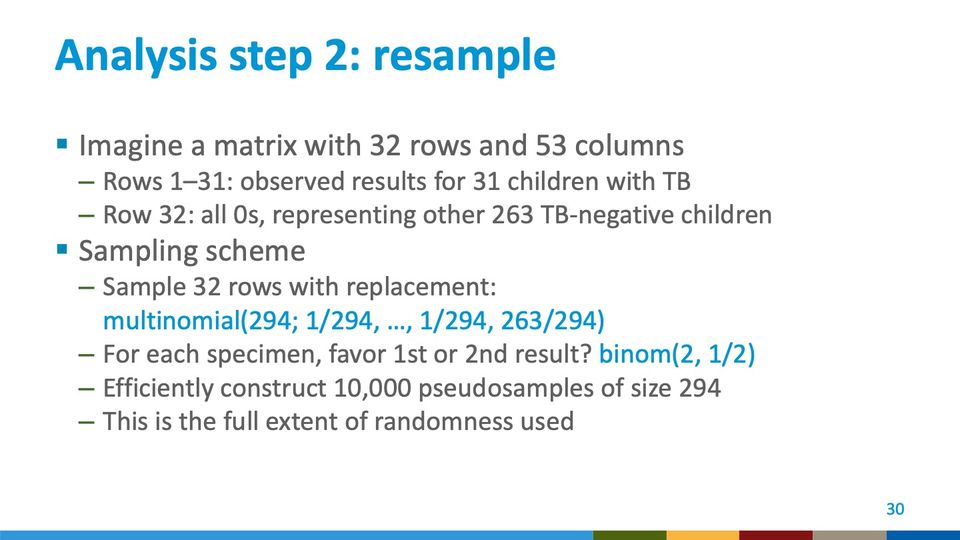
Abbreviations: TB = tuberculosis.
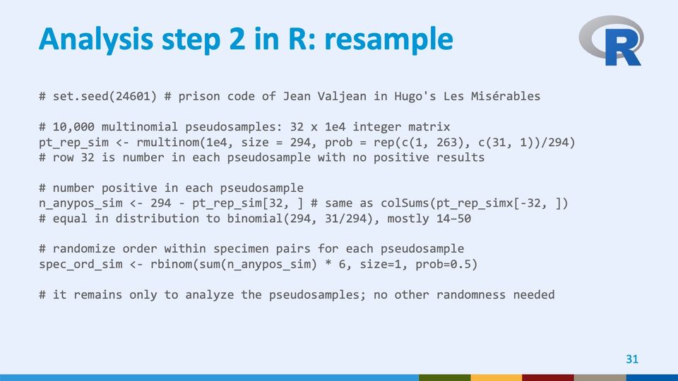
https://en.wikipedia.org/wiki/24,601 “It is the first prison code of the character Jean Valjean in the novel (his only code in the musical) Les Misérables. It was chosen by Victor Hugo when he believed that he was conceived on 24 June 1801 (that is, 24-6-01).” The other code is 9430. https://en.wikipedia.org/wiki/Jean_Valjean
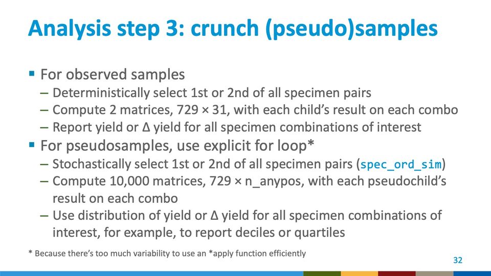
- Panels
- 1
- Elements
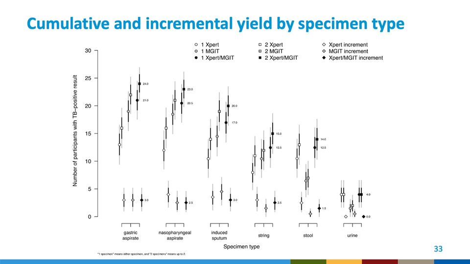
- 6 groups of 9 point markers, each marker with a thick black inner interval and a thinner light gray outer interval; marker shape and fill per legend: circles for 1 Xpert (white), 1 MGIT (gray), 1 Xpert/MGIT (black); squares for 2 Xpert (white), 2 MGIT (gray), 2 Xpert/MGIT (black); diamonds for Xpert increment (white), MGIT increment (gray), Xpert/MGIT increment (black). Within each group, circle-square pairs sit side by side at 3 tick positions (white, gray, black) with the diamonds below them; numeric labels beside the black markers; legend in 3 columns across the top
- Horizontal
- 6 specimen-type categories, each with a 3-tick bracket: gastric aspirate, nasopharyngeal aspirate, induced sputum, string, stool, urine; axis title Specimen type
- Vertical
- 0 to 30, ticks every 5; axis title Number of participants with TB–positive result
- Visible pattern
- The circle and square markers are highest for gastric and nasopharyngeal aspirate (black squares about 23 to 24), lower for induced sputum (about 20), lower again for string and stool (about 14 to 15), and lowest for urine, where all markers cluster between 0 and about 4. In stool the gray markers sit well below the white and black ones, at about 6 to 7. The increment diamonds lie along the bottom of every group, between 0 and about 5.
Text in the picture
24.0 21.0 3.0
23.0 20.5 2.5
20.0 17.0 3.0
15.0 12.5 2.5
14.0 12.5 1.5
4.0 0.0
"1 specimen" means either specimen, and "2 specimens" means up to 2.
Abbreviations: MGIT = Mycobacteria Growth Indicator Tube (liquid culture system); TB = tuberculosis; Xpert = Xpert MTB/RIF (Cepheid GeneXpert cartridge nucleic acid amplification test for TB and rifampicin resistance).
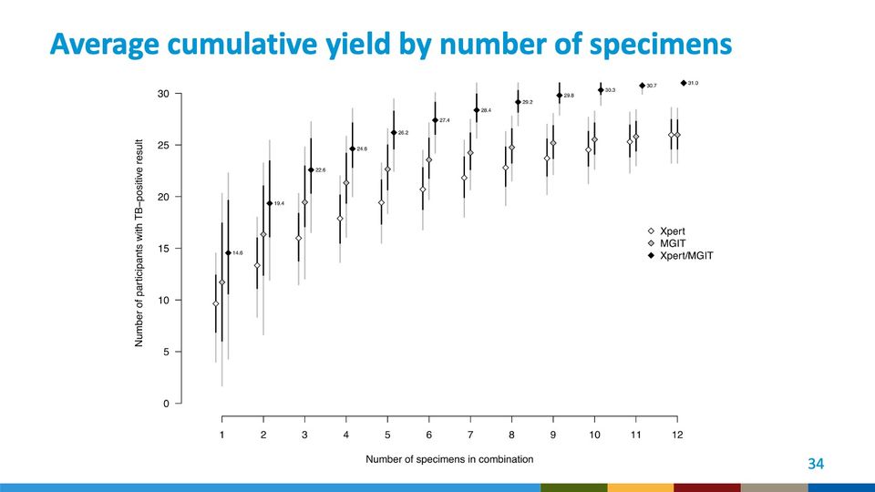
- Panels
- 1
- Elements
- 12 triplets of diamonds, white (Xpert), gray (MGIT) and black (Xpert/MGIT) per legend at right, each with a thick black inner interval and a thinner light gray outer interval; numeric labels beside the black diamonds
- Horizontal
- Number of specimens in combination, 1 to 12
- Vertical
- 0 to 30, ticks every 5; axis title Number of participants with TB–positive result; the black diamonds and their intervals extend above the top tick to about 31
- Visible pattern
- All 3 series rise from left to right, steeply over the first few specimens and then flattening. Black stays above gray, and gray above or level with white, throughout: black from about 15 to 31, gray from about 12 to 26, white from about 10 to 26, with white and gray meeting at about 26 at 12 specimens. Intervals are widest at 1 specimen, where the gray outer interval spans roughly 2 to 20, and narrow steadily to the right; at 12 specimens the black diamond shows no interval.
Text in the picture
14.6 19.4 22.6 24.6 26.2 27.4 28.4 29.2 29.8 30.3 30.7 31.0
Abbreviations: MGIT = Mycobacteria Growth Indicator Tube (liquid culture system); TB = tuberculosis; Xpert = Xpert MTB/RIF (Cepheid GeneXpert cartridge nucleic acid amplification test for TB and rifampicin resistance).
Text in the picture
CATS: ALL YOUR BASE R BELONG
TO US.
Text in the picture
www.cdc.gov
Abbreviations: CDC = Centers for Disease Control and Prevention; HHS = Department of Health and Human Services.
Text in the picture
I LOVE IT WHEN
YOU CALL ME BIG DATA
Abbreviations
CDC = Centers for Disease Control and Prevention; CI = contact investigation; DSS = demographic surveillance system; Dx = diagnosis; FM = fluorescence microscopy; FNA = fine-needle aspirate (of a lymph node); GA = gastric aspirate; GSUs = geographic study units; HC = health-facility enhancement plus contact investigation (trial condition H + C); HCM = health-facility enhancement plus contact investigation plus mobile unit (trial condition H + C + M); HF = health facility; HHS = Department of Health and Human Services; HIV = human immunodeficiency virus; HIV+ = HIV-positive; HM = health-facility enhancement plus mobile unit (trial condition H + M); IS = induced sputum; ISO = International Organization for Standardization; MGIT = Mycobacteria Growth Indicator Tube (liquid culture system); MU = mobile unit; NPA = nasopharyngeal aspirate; ST = string test (specimen collection method); TB = tuberculosis; Xpert = Xpert MTB/RIF (Cepheid GeneXpert cartridge nucleic acid amplification test for TB and rifampicin resistance).
References, compiled for this page
Full citations, with current links, for selected references and related works.
- Song R, Click ES, McCarthy KD, Heilig CM, Mchembere W, Smith JP, Fajans M, Musau SK, Okeyo E, Okumu A, et al. Sensitive and feasible specimen collection and testing strategies for diagnosing tuberculosis in young children. JAMA Pediatr. 2021;175(5):e206069. DOI 10.1001/jamapediatrics.2020.6069.
- Yuen CM, Agaya J, Mchembere W, Okelloh D, Achola M, Opole J, Cowden J, Heilig CM, Borgdorff MW, Cain KP. Optimizing the efficiency of tuberculosis active case-finding in health facilities and communities. Int. J. Tuberc. Lung Dis. 2019;23(7):844–849. DOI 10.5588/ijtld.18.0700.