Chad Heilig — CSELS Data Hub Webinar, 2018-11-19 — 77 slides
This rendering was constructed from an original PowerPoint presentation. Corrections of original text are indicated as “[corrected: X]”, redactions as “[redacted: X]”, and names withheld as “[generalized: X]”. Handouts and other auxiliary sources mentioned in the presentations are not available. The content of each presentation was believed to be correct and valid at the time of the presentation. This content, including references and links within the slides, has not been checked or updated when preparing this site. This rendering was facilitated by Anthropic Claude agentic tools for automated text extraction through computer vision and for assistance with compiling the completed sets.
Setting: Machine learning for public health—a primer, 2018-11-19. CDC’s Data Hub.
I presented “Machine Learning for Public Health—a Primer” to CDC staff on 2018-11-19 in a seminar sponsored by CDC’s Data Hub, a service of the Division for Health Informatics and Surveillance in the Center for Surveillance, Epidemiology, and Laboratory Services. Scott Lee and I planned a pair of seminars. Scott led a companion workshop on 12-14 in which he demonstrated a mix of Python and R code for analyzing publicly available data using 5 of the methods presented in the 11-19 seminar. Scott is lead author on papers that apply machine learning, one of which continues Matt Maenner’s work on autism surveillance. We continued presenting this work to CDC’s Data Science Upskilling program, the Office of the Chief Science Officer and the High-Performance Computing Subcommittee, the Statistical and Machine Learning Community of Practice, and several college and university audiences.
Slide 1Machine Learning for Public Health. —a Primer
Chad Heilig, PhD • [redacted: email address] Scott Lee, PhD • [redacted: email address] CSELS Machine Learning • [redacted: email address] CSELS Data Hub Webinar, 2018-11-19
Description
Text in the picture
data hub
Abbreviations: CSELS = Center for Surveillance, Epidemiology, and Laboratory Services (CDC).
Slide 2Origins and Acknowledgments
2015 Jeff Dean (Langmuir), Ventures/iFund
2018 Statistics Day
CSELS/DHIS Data Hub
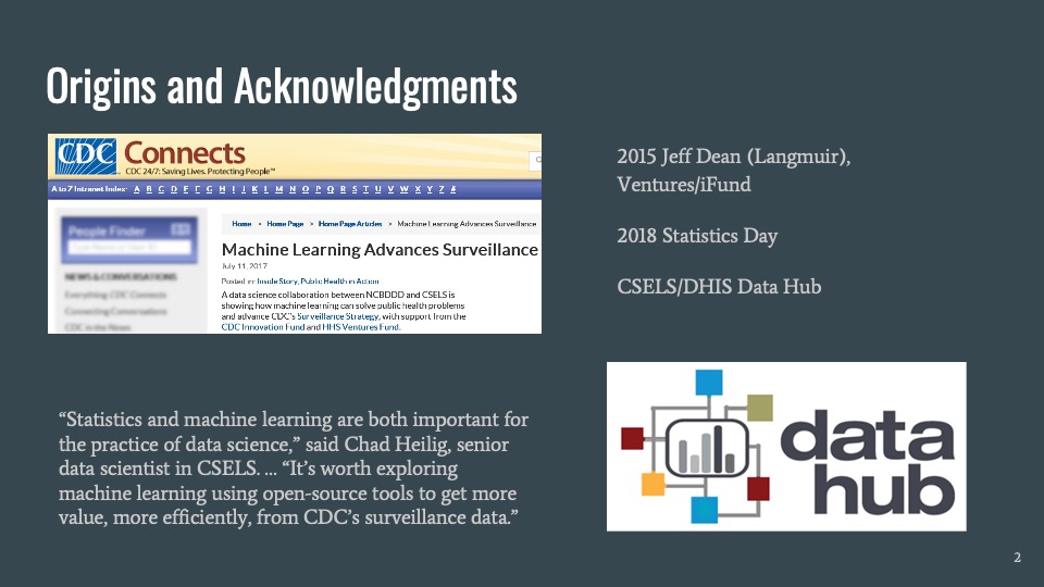
[redacted: intranet URL] machine-learning-advances-surveillance/ “Statistics and machine learning are both important for the practice of data science,” said Chad Heilig, senior data scientist in CSELS. … “It’s worth exploring machine learning using open-source tools to get more value, more efficiently, from CDC’s surveillance data.”
Description
A screenshot of an intranet page, containing CDC logo and the name CDC Connects, site chrome, and a partially redacted excerpt of a Connects article. The Data Hub logo sits at lower right, as on the title slide.
Text in the picture
Machine Learning Advances Surveillance Machine Learning Advances Surveillance July 11, 2017 Posted in: Inside Story, Public Health in Action A data science collaboration between NCBDDD and CSELS is showing how machine learning can solve public health problems and advance CDC's Surveillance Strategy, with support from the CDC Innovation Fund and HHS Ventures Fund.
Presenter notes
[redacted: intranet URL]
Abbreviations: CDC = Centers for Disease Control and Prevention; CSELS = Center for Surveillance, Epidemiology, and Laboratory Services (CDC); DHIS = Division of Health Informatics and Surveillance (CDC, in CSELS); HHS = Department of Health and Human Services; NCBDDD = National Center on Birth Defects and Developmental Disabilities (CDC).
Slide 3Purpose and scope
Build intuition for machine learning through public health examples
Public health context: What’s the question to which ML is applied?
Machine learning context: How does ML answer the question? Why ML?
Data-analytic concepts: Explain and demystify through these examples
Scope is limited by time and purpose
Focus on data-analytic applications
Won’t go deep; won’t go mathy (no formulae)
Mention other-than-analytic examples (“artificial intelligence”) in passing
Many, many other applications and methods, even in public health
Presenter notes
[mention daily “programmatic” uses: web search suggestions, item recommendations, facial tagging / image search, natural language understanding and translation] Main concepts of machine learning for data analysis Demystify, build nontechnical intuition Pointers to examples, tools for further learning and experience Data Hub, SharePoint, and Git resources; annotated bibliography December 14 hands-on seminar: worked examples in Python and R
Abbreviations: ML = machine learning.
Slide 40. Machine learning: panacea (umm, no)
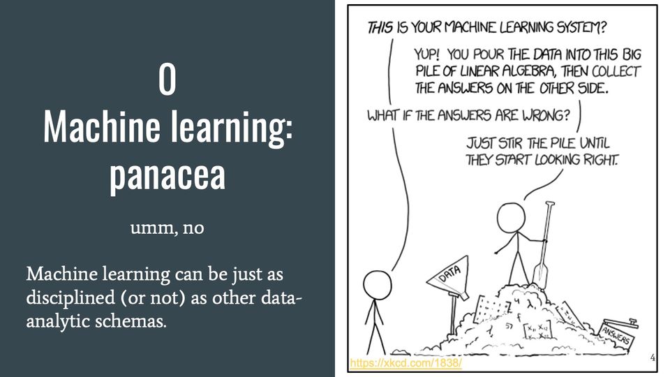
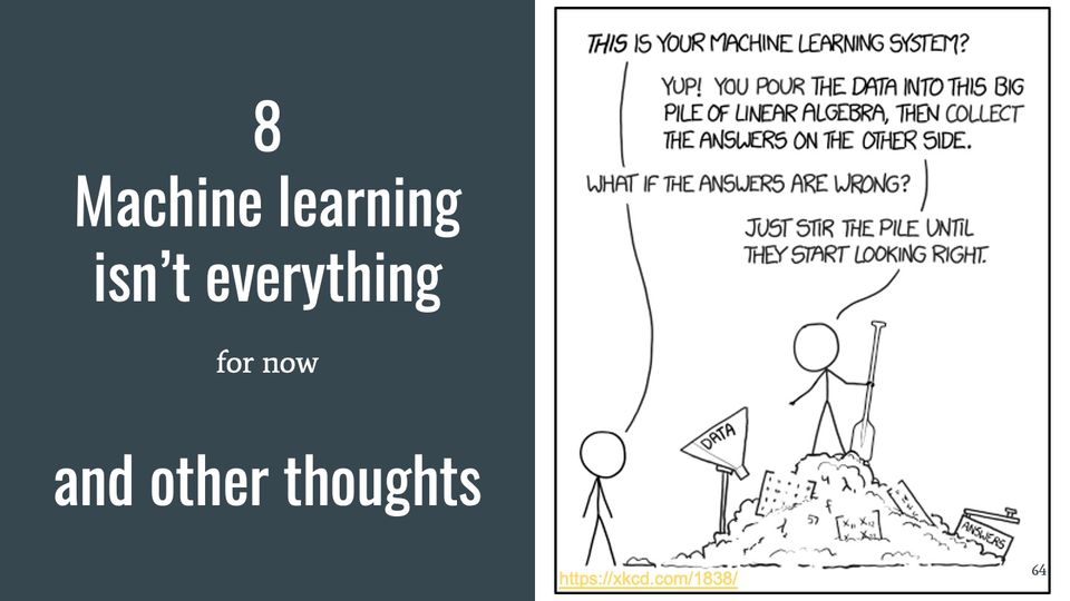
umm, no Machine learning can be just as disciplined (or not) as other data-analytic schemas.
A four-line exchange in which one figure questions the machine learning system and the other explains how it works and what to do when its answers are wrong.
Presenter notes
https://xkcd.com/1838/ Transcript [Cueball Prime, holds a canoe paddle at his side and stands on top of a "big pile of linear algebra" containing a funnel labeled "data" and box labeled "answers". Cueball II stands to the left side of the panel.)] Cueball II: This is your machine learning system? Cueball Prime: Yup! You pour the data into this big pile of linear algebra, then collect the answers on the other side. Cueball II: What if the answers are wrong? Cueball Prime: Just stir the pile until they start looking right.
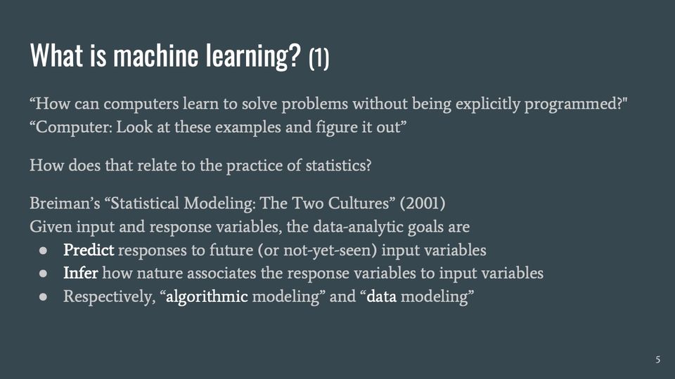
Slide 5What is machine learning? (1)
“How can computers learn to solve problems without being explicitly programmed?"
“Computer: Look at these examples and figure it out”
How does that relate to the practice of statistics?
Breiman’s “Statistical Modeling: The Two Cultures” (2001)
Given input and response variables, the data-analytic goals are
Predict responses to future (or not-yet-seen) input variables
Infer how nature associates the response variables to input variables
Respectively, “algorithmic modeling” and “data modeling”
Presenter notes
https://en.wikipedia.org/wiki/Machine_learning#References Samuel, Arthur (1959). "Some Studies in Machine Learning Using the Game of Checkers". IBM Journal of Research and Development. 3 (3): 210–229. CiteSeerX 10.1.1.368.2254. doi:10.1147/rd.33.0210. "Paraphrasing Arthur Samuel (1959), the question is: How can computers learn to solve problems without being explicitly programmed?" in Koza, John R.; Bennett, Forrest H.; Andre, David; Keane, Martin A. (1996). Automated Design of Both the Topology and Sizing of Analog Electrical Circuits Using Genetic Programming. Artificial Intelligence in Design '96. Springer, Dordrecht. pp. 151–170. doi:10.1007/978-94-009-0279-4_9. Jonathan Chen, Stanford Presence AIMIE 2018-08-22 https://www.youtube.com/watch?v=2r_C3dMZuSE Breiman L. Statistical modeling: The two cultures. Statistical Science. 2001;16(3):199-231. https://projecteuclid.org/euclid.ss/1009213726
Abbreviations: AIMIE = AI in Medicine: Inclusion & Equity symposium; IBM = individual-based model.
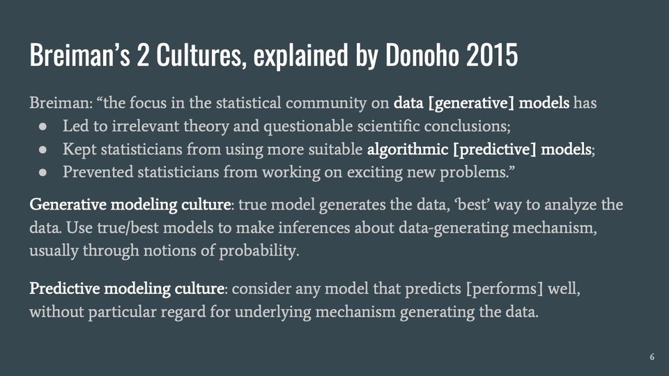
Slide 6Breiman’s 2 Cultures, explained by Donoho 2015
Breiman: “the focus in the statistical community on data [generative] models has
Led to irrelevant theory and questionable scientific conclusions;
Kept statisticians from using more suitable algorithmic [predictive] models;
Prevented statisticians from working on exciting new problems.”
Generative modeling culture: true model generates the data, ‘best’ way to analyze the data. Use true/best models to make inferences about data-generating mechanism, usually through notions of probability.
Predictive modeling culture: consider any model that predicts [performs] well, without particular regard for underlying mechanism generating the data.
Presenter notes
Donoho D. 50 years of data science. Journal of Computational and Graphical Statistics. 2017 Oct 2;26(4):745-66. https://doi.org/10.1080/10618600.2017.1384734 [Open Access] “predict” means anticipate a not-yet-seen target value based on inputs, not necessarily forecast the future
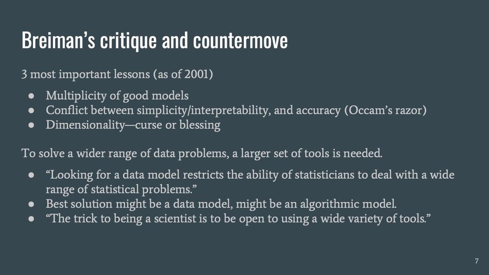
Slide 7Breiman’s critique and countermove
3 most important lessons (as of 2001)
Multiplicity of good models
Conflict between simplicity/interpretability, and accuracy (Occam’s razor)
Dimensionality—curse or blessing
To solve a wider range of data problems, a larger set of tools is needed.
“Looking for a data model restricts the ability of statisticians to deal with a wide range of statistical problems.”
Best solution might be a data model, might be an algorithmic model.
“The trick to being a scientist is to be open to using a wide variety of tools.”
Presenter notes
many models, possibly dissimilar from each other, can perform similarly well; this is OK [note: also more OK in statistics than it was in 2001, as in bayesian model averaging] parsimony and interpretability are heuristics that don’t generally have strong procedural support, though they can admit some narrowly constructed mathematical proofs
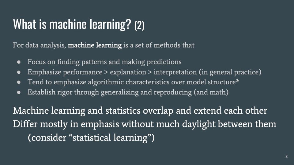
Slide 8What is machine learning? (2)
For data analysis, machine learning is a set of methods that
Focus on finding patterns and making predictions
Emphasize performance > explanation > interpretation (in general practice)
Tend to emphasize algorithmic characteristics over model structure*
Establish rigor through generalizing and reproducing (and math)
Machine learning and statistics overlap and extend each other
Differ mostly in emphasis without much daylight between them
(consider “statistical learning”)
Presenter notes
* model structure is important (e.g., NN architectures), but for performance rather than to capture or explain data structure
Abbreviations: NN = neural network.
Slide 9Some useful machine learning vocabulary
Task: the (kind of) problem that you want to solve: segment groups, classify new example, predict timing or size of an event, generate synthetic data
Model: the method for using data to achieve a task: spline regression, random forest, support vector machine, neural network; evaluated by performance
Feature: representation (possibly derived) of data that models operate on: continuous variable, indicator, count of word frequencies
Train/learn, validate, test: fit a model, refine some parameters, check on unseen data
Unsupervised, supervised learning: find structure vs relate an output to inputs
(examples …)
Presenter notes
Flach, Peter A. 2017. Machine learning: the art and science of algorithms that make sense of data. Cambridge: Cambridge University Press. ISBN 9781107422223 unsupervised examples: cluster analysis, feature selection (e.g., CMIM), dimension reduction (e.g., PCA) supervised examples: classification, regression
Abbreviations: CMIM = conditional mutual information maximization (a feature-selection method); ISBN = International Standard Book Number; PCA = principal component analysis.
Slide 10Some uses of machine learning at CDC/ATSDR
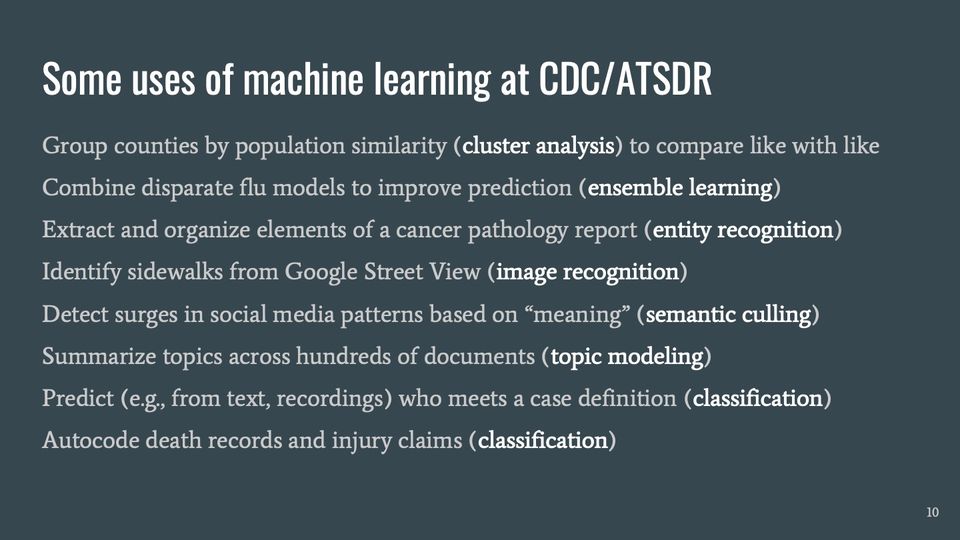
Group counties by population similarity (cluster analysis) to compare like with like
Combine disparate flu models to improve prediction (ensemble learning)
Extract and organize elements of a cancer pathology report (entity recognition)
Identify sidewalks from Google Street View (image recognition)
Detect surges in social media patterns based on “meaning” (semantic culling)
Summarize topics across hundreds of documents (topic modeling)
Predict (e.g., from text, recordings) who meets a case definition (classification)
Autocode death records and injury claims (classification)
Presenter notes
Group counties by similarity (cluster analysis) to compare like with like: CSELS/DPHID’s former CHSI Combine disparate flu models to improve prediction (ensemble learning): FluSight, NCIRD/ID Extract and organize elements of a cancer pathology report (entity recognition): NCCDPHP/DCPC Identify sidewalks from Google Street View (image recognition): NCCDPHP/DNPAO Detect surges in social media patterns based on “meaning” (semantic culling): [corrected: CPR]/DEO, NCIPC Summarize topics across hundreds of documents (topic modeling): OPHSS Predict (e.g., from text, recordings) who meets a case definition (classification): NCBDDD Autocode death records and injury claims (classification): NCHS, NIOSH
Abbreviations: ATSDR = Agency for Toxic Substances and Disease Registry; CDC = Centers for Disease Control and Prevention; CHSI = Community Health Status Indicators; CPR = Center for Preparedness and Response (CDC); CSELS = Center for Surveillance, Epidemiology, and Laboratory Services (CDC); DCPC = Division of Cancer Prevention and Control (CDC/NCCDPHP); DEO = Division of Emergency Operations (CDC); DNPAO = Division of Nutrition, Physical Activity, and Obesity (CDC/NCCDPHP); DPHID = Division of Public Health Information Dissemination (CDC/CSELS); NCBDDD = National Center on Birth Defects and Developmental Disabilities (CDC); NCCDPHP = National Center for Chronic Disease Prevention and Health Promotion (CDC); NCHS = National Center for Health Statistics (CDC); NCIPC = National Center for Injury Prevention and Control (CDC); NCIRD = National Center for Immunization and Respiratory Diseases (CDC); NIOSH = National Institute for Occupational Safety and Health (CDC); OPHSS = Office of Public Health Scientific Services (CDC).
Slide 11The remainder of this talk
Structure of this talk evolved over the 2 months of planning
Was going to be a set of concepts, defined, with examples where possible
Reviewed ~100 manuscripts that mention machine learning and
either mention public health
or include a CDC/ATSDR-affiliated author
Whirlwind tour of 7 kinds of applications (15 manuscripts),
how to interpret them (in < 60 minutes), punctuated by commentary
(Annotated bibliography will be made available on SharePoint)
Presenter notes
[redacted: intranet URL] [redacted: intranet URL] About 58 manuscripts cover the 7 domains
Abbreviations: ATSDR = Agency for Toxic Substances and Disease Registry; CDC = Centers for Disease Control and Prevention.
this section: for a given model type (e.g., straight lines), how to select best model of that type (minimize error or maximize likelihood) -- implicit comparison of all possible straight lines with a single predictor; selection is usually based on internal criteria (fit) rather than external (predictive performance; here’s where error especially comes in) for a given model type, extend to multiple predictors -- this leads us into feature selection (e.g., forward selection, backward elimination, stepwise regression, best subset regression) -- dangers: overfitting, poor prediction; one guard: cross-validation what if we extend the model types, to bend to the data?
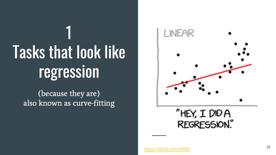
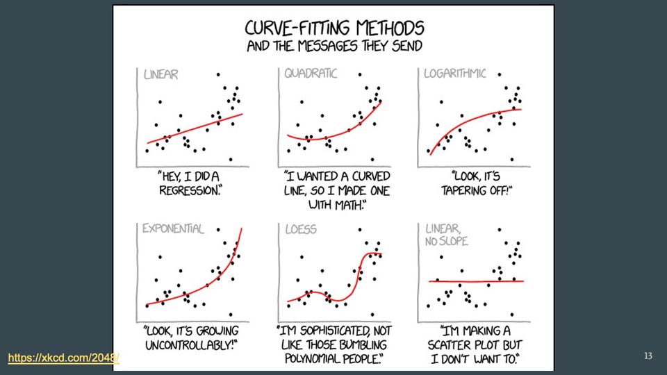
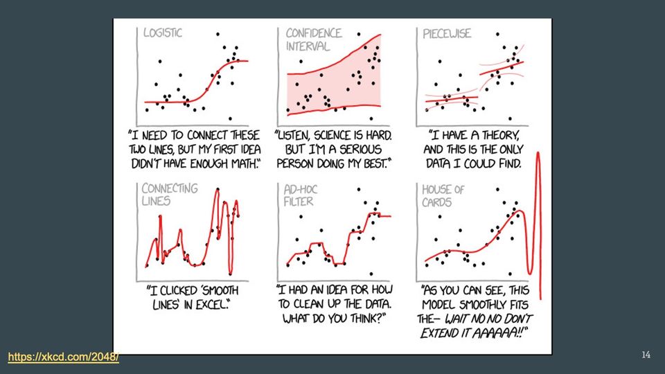
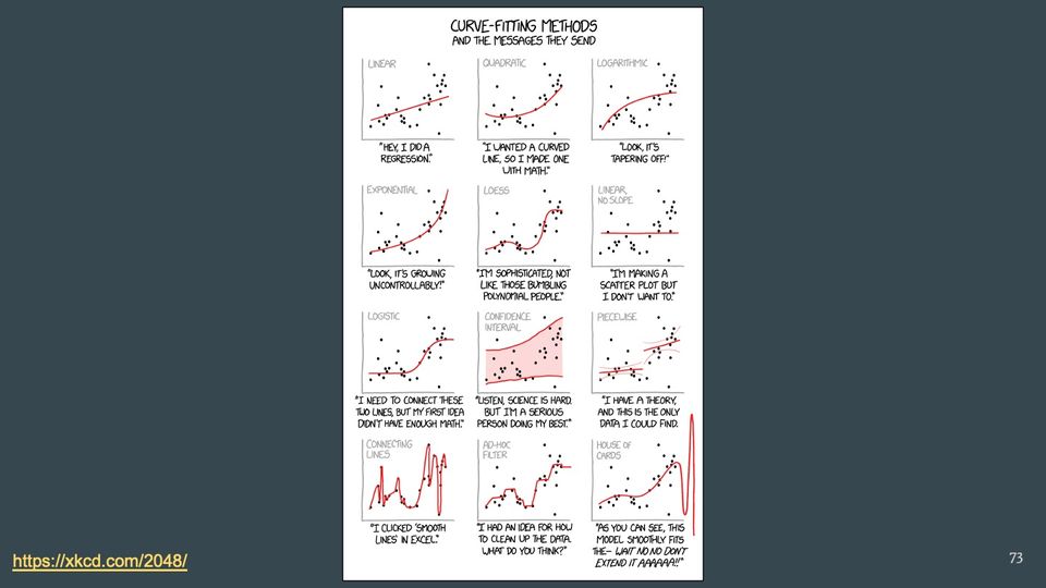
https://xkcd.com/2048/ Curve-Fitting Methods, part 1 extending model types: linear has 2 parameters (intercept and slope); quadratic adds curvature and an additional parameter; logarithmic and exponential also have 2 parameters; no-slope model has only 1 (constant = mean of vertical values) loess is fancier, and it entails some tradeoffs between goodness-of-fit (or prediction) and smoothness; correspond to tradeoff in bias and variance, between complexity and generalizability
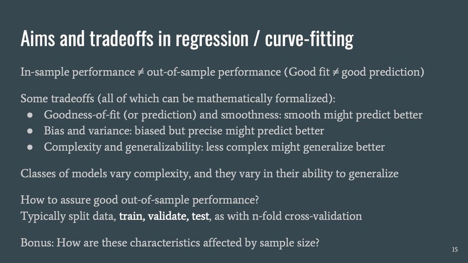
Slide 15Aims and tradeoffs in regression / curve-fitting
In-sample performance ≠ out-of-sample performance (Good fit ≠ good prediction)
Some tradeoffs (all of which can be mathematically formalized):
Goodness-of-fit (or prediction) and smoothness: smooth might predict better
Bias and variance: biased but precise might predict better
Complexity and generalizability: less complex might generalize better
Classes of models vary complexity, and they vary in their ability to generalize
How to assure good out-of-sample performance?
Typically split data, train, validate, test, as with n-fold cross-validation
Bonus: How are these characteristics affected by sample size?
Presenter notes
several methods for assuring out-of-sample performance: single split, leave-1-out (closed solution in linear regression), gather new data more data: less bias (if estimator is consistent), less variance, easier to train/validate/test
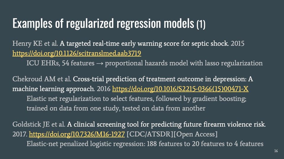
Slide 16Examples of regularized regression models (1)
Elastic net regularization to select features, followed by gradient boosting;
trained on data from one study, tested on data from another
Goldstick JE et al. A clinical screening tool for predicting future firearm violence risk. 2017. https://doi.org/10.7326/M16-1927 [CDC/ATSDR][Open Access]
Elastic-net penalized logistic regression: 188 features to 20 features to 4 features
Abbreviations: ATSDR = Agency for Toxic Substances and Disease Registry; CDC = Centers for Disease Control and Prevention; EHR = electronic health record; ICU = intensive care unit; KE = Kenya.
Slide 17What is feature selection?
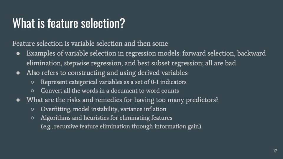
Feature selection is variable selection and then some
Examples of variable selection in regression models: forward selection, backward elimination, stepwise regression, and best subset regression; all are bad
Also refers to constructing and using derived variables
Represent categorical variables as a set of 0-1 indicators
Convert all the words in a document to word counts
What are the risks and remedies for having too many predictors?
Overfitting, model instability, variance inflation
Algorithms and heuristics for eliminating features
(e.g., recursive feature elimination through information gain)
Slide 18What is regularized regression?
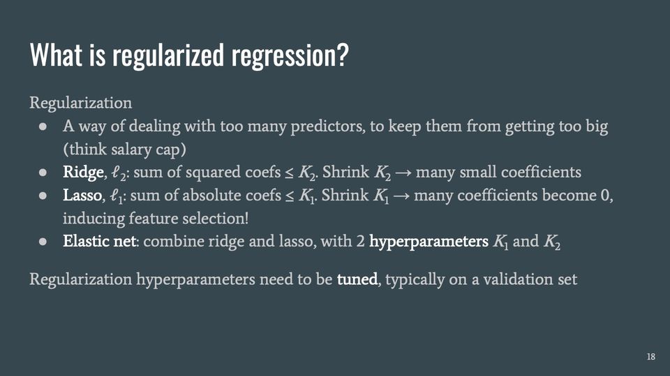
Regularization
A way of dealing with too many predictors, to keep them from getting too big (think salary cap)
Ridge, ℓ2: sum of squared coefs ≤ K2. Shrink K2 → many small coefficients
Lasso, ℓ1: sum of absolute coefs ≤ K1. Shrink K1 → many coefficients become 0, inducing feature selection!
Elastic net: combine ridge and lasso, with 2 hyperparameters K1 and K2
Regularization hyperparameters need to be tuned, typically on a validation set
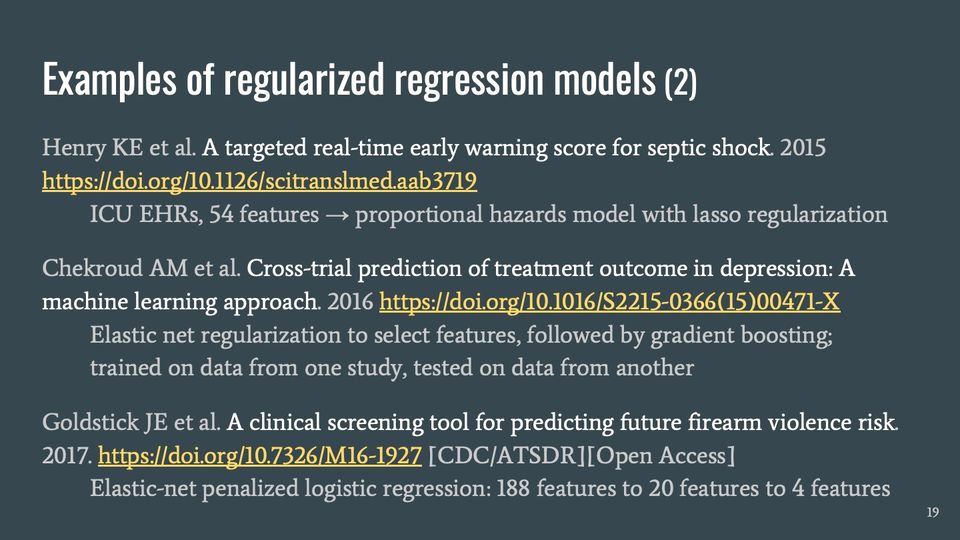
Slide 19Examples of regularized regression models (2)
Elastic net regularization to select features, followed by gradient boosting;
trained on data from one study, tested on data from another
Goldstick JE et al. A clinical screening tool for predicting future firearm violence risk. 2017. https://doi.org/10.7326/M16-1927 [CDC/ATSDR][Open Access]
Elastic-net penalized logistic regression: 188 features to 20 features to 4 features
Abbreviations: ATSDR = Agency for Toxic Substances and Disease Registry; CDC = Centers for Disease Control and Prevention; EHR = electronic health record; ICU = intensive care unit; KE = Kenya.
Slide 20Further comments on regression-based methods
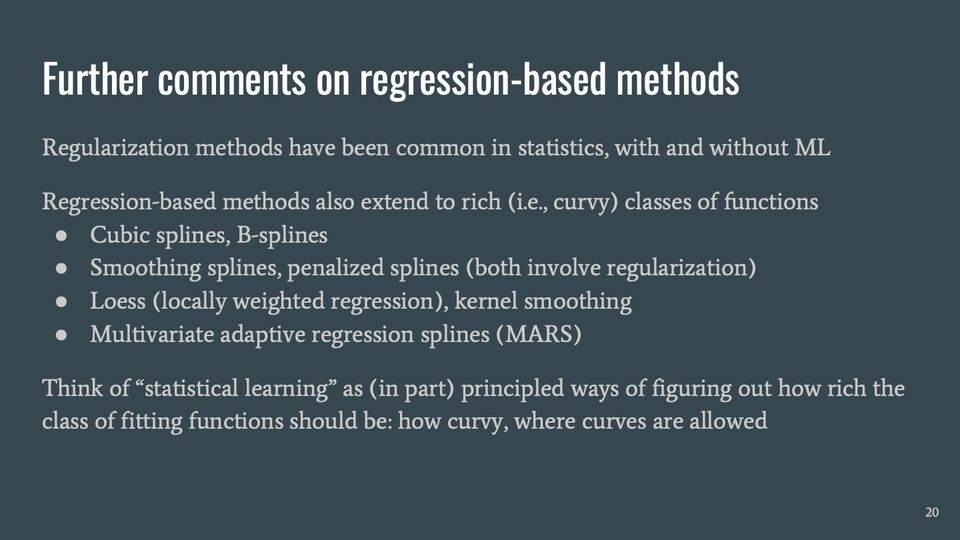
Regularization methods have been common in statistics, with and without ML
Regression-based methods also extend to rich (i.e., curvy) classes of functions
Think of “statistical learning” as (in part) principled ways of figuring out how rich the class of fitting functions should be: how curvy, where curves are allowed
Abbreviations: MARS = multivariate adaptive regression splines; ML = machine learning.
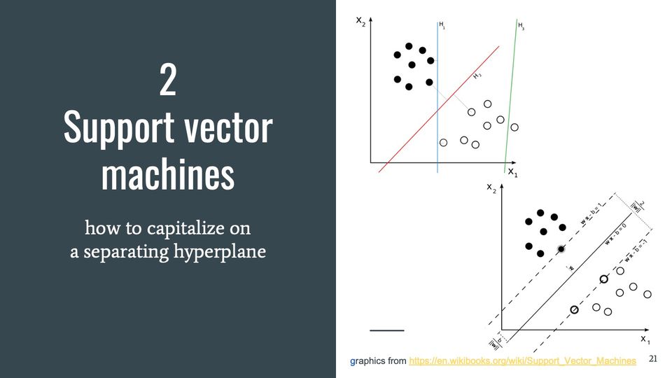
[graphic of filled and unfilled dots, separated by 3 lines: H3 separates 1 unfilled dot from all other dots; H1 separates filled from unfilled dots; H2 maximally separates filled from unfilled dots]
[graphic of filled maximally separated filled from unfilled dots; further explained on Slides 23 and 24]
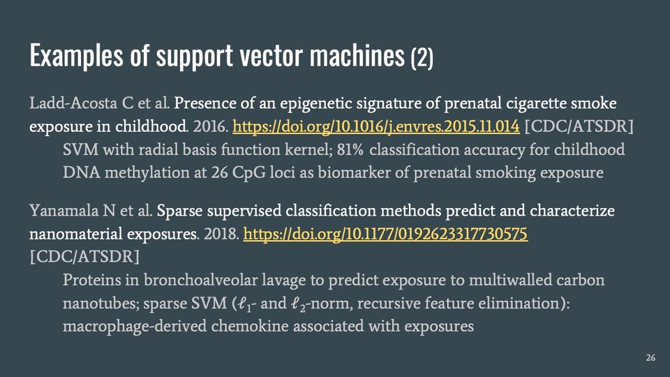
SVM with radial basis function kernel; 81% classification accuracy for childhood DNA methylation at 26 CpG loci as biomarker of prenatal smoking exposure
Yanamala N et al. Sparse supervised classification methods predict and characterize nanomaterial exposures. 2018. https://doi.org/10.1177/0192623317730575 [CDC/ATSDR]
Proteins in bronchoalveolar lavage to predict exposure to multiwalled carbon nanotubes; sparse SVM (ℓ1- and ℓ2-norm, recursive feature elimination): macrophage-derived chemokine associated with exposures
Abbreviations: ATSDR = Agency for Toxic Substances and Disease Registry; CDC = Centers for Disease Control and Prevention; CpG = CpG (cytosine–phosphate–guanine) site; DNA = deoxyribonucleic acid; SVM = support vector machine.
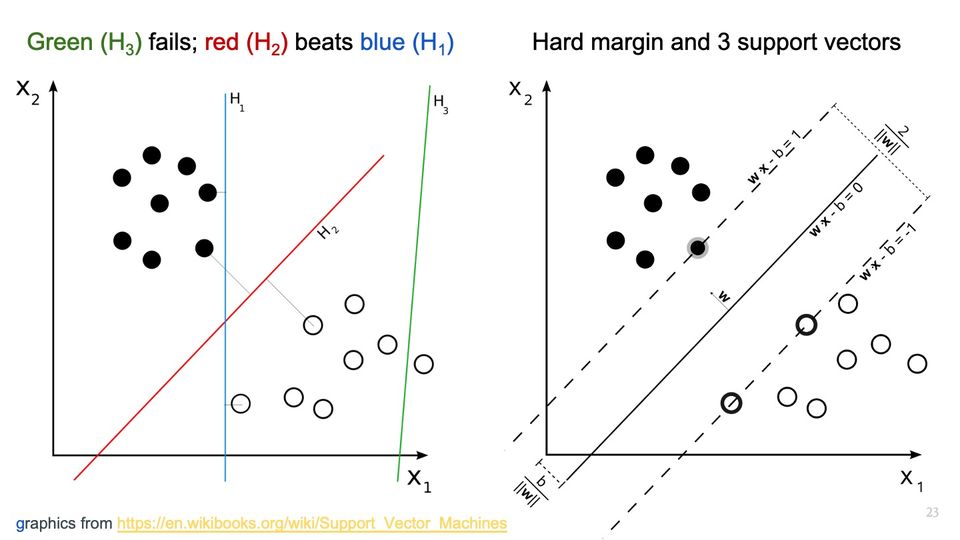
[graphic of filled and unfilled dots, separated by 3 lines: H3 separates 1 unfilled dot from all other dots; H1 separates filled from unfilled dots; H2 maximally separates filled from unfilled dots]
[graphic of filled maximally separated filled from unfilled dots; further explained on Slide 24]
The simplest support vector classifier separates 2 sets of points by cutting between them, with maximum separation (maximal margin classifier)
Separating hyperplane is the (hard) margin; points at the margin are support vectors
If points can only be approximately linearly separated, a soft margin is found
Penalty hyperparameter for misclassified points on the wrong side of margin, hence some tuning is needed
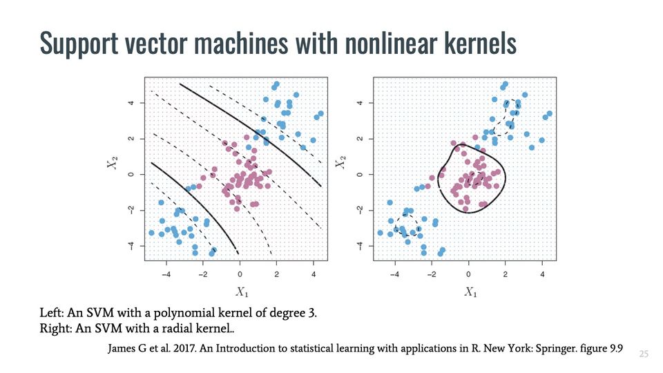
Kernel trick extends linear separation through a rich set of separating curves
Slide 25Support vector machines with nonlinear kernels
Support vector machines with nonlinear kernels
Left: An SVM with a polynomial kernel of degree 3. Right: An SVM with a radial kernel.. James G et al. 2017. An Introduction to statistical learning with applications in R. New York: Springer. figure 9.9
SVM with radial basis function kernel; 81% classification accuracy for childhood DNA methylation at 26 CpG loci as biomarker of prenatal smoking exposure
Yanamala N et al. Sparse supervised classification methods predict and characterize nanomaterial exposures. 2018. https://doi.org/10.1177/0192623317730575 [CDC/ATSDR]
Proteins in bronchoalveolar lavage to predict exposure to multiwalled carbon nanotubes; sparse SVM (ℓ1- and ℓ2-norm, recursive feature elimination): macrophage-derived chemokine associated with exposures
Abbreviations: ATSDR = Agency for Toxic Substances and Disease Registry; CDC = Centers for Disease Control and Prevention; CpG = CpG (cytosine–phosphate–guanine) site; DNA = deoxyribonucleic acid; SVM = support vector machine.
Slide 27Further comments on support vector machines
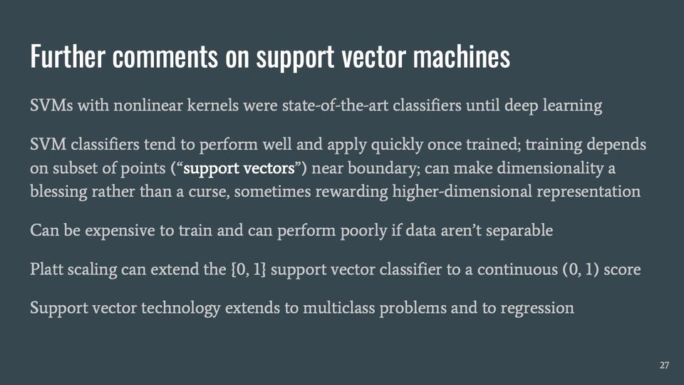
SVMs with nonlinear kernels were state-of-the-art classifiers until deep learning
SVM classifiers tend to perform well and apply quickly once trained; training depends on subset of points (“support vectors”) near boundary; can make dimensionality a blessing rather than a curse, sometimes rewarding higher-dimensional representation
Can be expensive to train and can perform poorly if data aren’t separable
Platt scaling can extend the {0, 1} support vector classifier to a continuous (0, 1) score
Support vector technology extends to multiclass problems and to regression
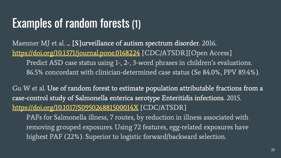
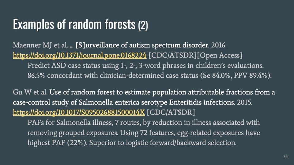
Predict ASD case status using 1-, 2-, 3-word phrases in children’s evaluations. 86.5% concordant with clinician-determined case status (Se 84.0%, PPV 89.4%).
Gu W et al. Use of random forest to estimate population attributable fractions from a case-control study of Salmonella enterica serotype Enteritidis infections. 2015. https://doi.org/10.1017/S095026881500014X [CDC/ATSDR]
PAFs for Salmonella illness, 7 routes, by reduction in illness associated with removing grouped exposures. Using 72 features, egg-related exposures have highest PAF (22%). Superior to logistic forward/backward selection.
Abbreviations: ASD = autism spectrum disorder; ATSDR = Agency for Toxic Substances and Disease Registry; CDC = Centers for Disease Control and Prevention; PAF = population attributable fraction; PPV = positive predictive value.
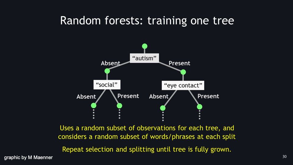
Slide 30Random forests: training one tree
graphic by M Maenner
Description
graphic of a single example tree (by M Maenner)
Random forests: training one tree
first split on word “autism”
if word “autism” is absent, go left; if present, go right
after going left, split on “social”; if absent, go left; if present go right; and so on
after going right, split on “eye contact”; if absent, go left; if present go right; and so on
Uses a random subset of observations for each tree, and considers a random subset of words/phrases at each split
Repeat selection and splitting until tree is fully grown.
Presenter notes
credit: Matt Maenner
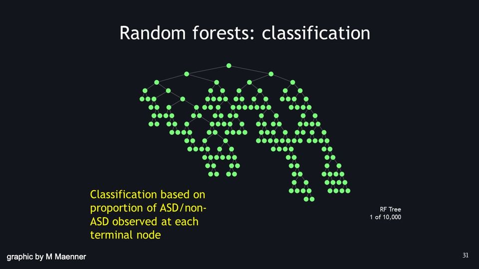
Slide 31Random forests: classification
graphic by M Maenner
Description
graphic of a single, fully grown tree (by M Maenner)
Random forests: classification
RF Tree 1 of 10,000
Classification based on proportion of ASD/non-ASD observed at each terminal node
Presenter notes
credit: Matt Maenner
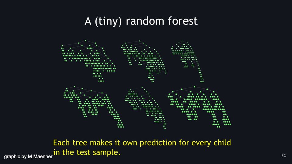
Slide 32A (tiny) random forest
graphic by M Maenner
Description
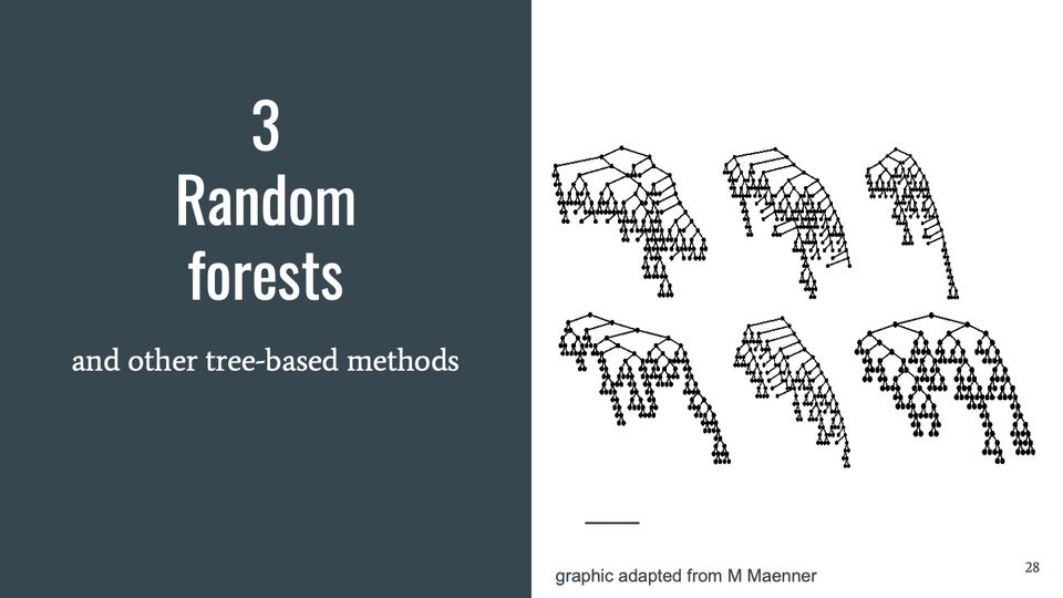
graphic of 6 fully grown trees (by M Maenner)
A (tiny) random forest
Each tree makes its own prediction for every child in the test sample.
Presenter notes
credit: Matt Maenner
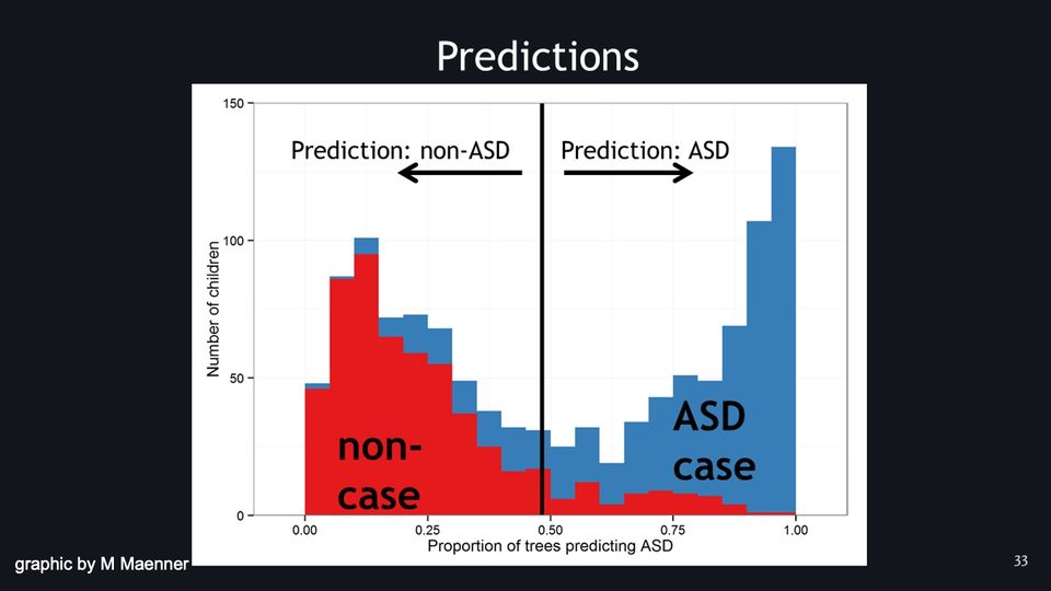
Slide 33Random forest predictions
graphic by M Maenner
Description
graphic o stacked histograms (by M Maenner)
vertical axis: number of children
horizontal axis: proportion of trees predicting ASD
left of 0.43 “prediction: noncase”; most, but not all, children with <0.43 fraction of trees predicting ASD are correctly classified as not cases; a small fraction are incorrectly classified (false negatives)
right of 0.43 “prediction: case”; most, but not all, children with >0.43 fraction of trees predicting ASD are correctly classified as cases; a small fraction are incorrectly classified (false positives)
Presenter notes
credit: Matt Maenner
Abbreviations: ASD = autism spectrum disorder.
Slide 34What are random forests?
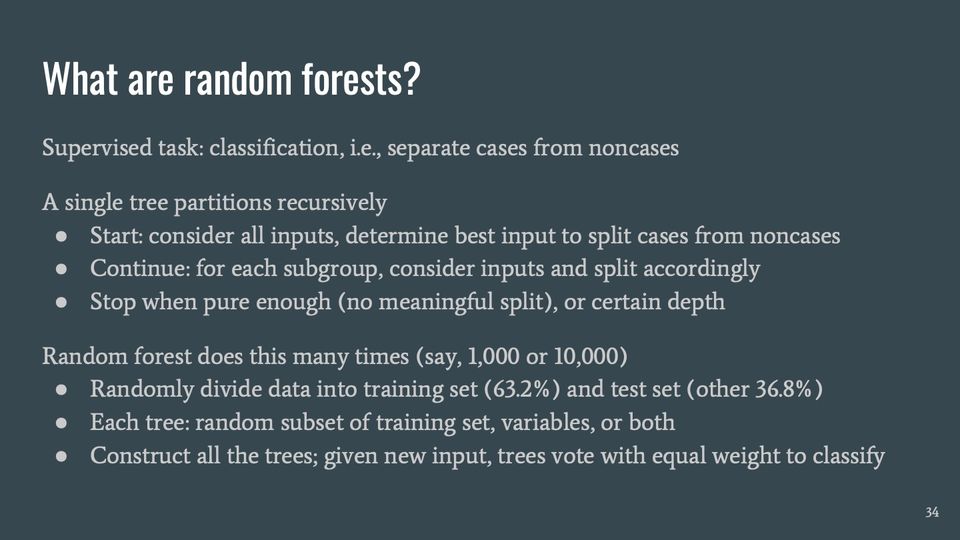
Supervised task: classification, i.e., separate cases from noncases
A single tree partitions recursively
Start: consider all inputs, determine best input to split cases from noncases
Continue: for each subgroup, consider inputs and split accordingly
Stop when pure enough (no meaningful split), or certain depth
Random forest does this many times (say, 1,000 or 10,000)
Randomly divide data into training set (63.2%) and test set (other 36.8%)
Each tree: random subset of training set, variables, or both
Construct all the trees; given new input, trees vote with equal weight to classify
Predict ASD case status using 1-, 2-, 3-word phrases in children’s evaluations. 86.5% concordant with clinician-determined case status (Se 84.0%, PPV 89.4%).
Gu W et al. Use of random forest to estimate population attributable fractions from a case-control study of Salmonella enterica serotype Enteritidis infections. 2015. https://doi.org/10.1017/S095026881500014X [CDC/ATSDR]
PAFs for Salmonella illness, 7 routes, by reduction in illness associated with removing grouped exposures. Using 72 features, egg-related exposures have highest PAF (22%). Superior to logistic forward/backward selection.
Abbreviations: ASD = autism spectrum disorder; ATSDR = Agency for Toxic Substances and Disease Registry; CDC = Centers for Disease Control and Prevention; PAF = population attributable fraction; PPV = positive predictive value.
Slide 36Further comments on tree-based methods (1)
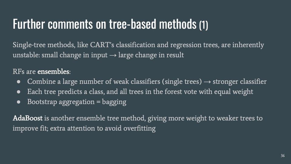
Single-tree methods, like CART’s classification and regression trees, are inherently unstable: small change in input → large change in result
RFs are ensembles:
Combine a large number of weak classifiers (single trees) → stronger classifier
Each tree predicts a class, and all trees in the forest vote with equal weight
Bootstrap aggregation = bagging
AdaBoost is another ensemble tree method, giving more weight to weaker trees to improve fit; extra attention to avoid overfitting
Presenter notes
[Compare with model averaging and importance sampling?]
Abbreviations: CART = classification and regression trees; RF = random forest.
Slide 37Further comments on tree-based methods (2)
More characteristics of random forests:
Fewer settings to tune compared to SVM or boosting
Built-in variable importance measures
Fairly robust to noninformative features; inherently resistant to overfitting
Out-of-bag error rate approximates error in validation sample
Presenter notes
credit: Matt Maenner
Abbreviations: SVM = support vector machine.
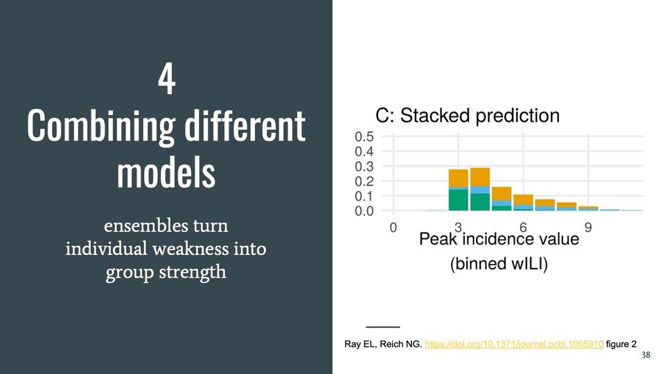
Slide 384. Combining different models
ensembles turn individual weakness into group strength
Ray EL, Reich NG. Prediction of infectious disease epidemics via weighted density ensembles. PLoS Computational Biology. 2018 Feb 20;14(2):e1005910. https://doi.org/10.1371/journal.pcbi.1005910 figure 2C, page 8
Slide 39Examples of ensemble methods (1)
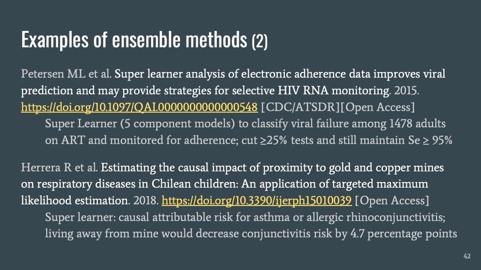
Petersen ML et al. Super learner analysis of electronic adherence data improves viral prediction and may provide strategies for selective HIV RNA monitoring. 2015. https://doi.org/10.1097/QAI.0000000000000548 [CDC/ATSDR][Open Access]
Super Learner (5 component models) to classify viral failure among 1478 adults on ART and monitored for adherence; cut ≥ 25% tests and still maintain Se ≥ 95%
Herrera R et al. Estimating the causal impact of proximity to gold and copper mines on respiratory diseases in Chilean children: An application of targeted maximum likelihood estimation. 2018. https://doi.org/10.3390/ijerph15010039 [Open Access]
Super learner: causal attributable risk for asthma or allergic rhinoconjunctivitis; living away from mine would decrease conjunctivitis risk by 4.7 percentage points
Abbreviations: ART = antiretroviral therapy; ATSDR = Agency for Toxic Substances and Disease Registry; CDC = Centers for Disease Control and Prevention; HIV = human immunodeficiency virus; ML = machine learning; RNA = ribonucleic acid.
Slide 40Stacking to create ensemble predictive distribution
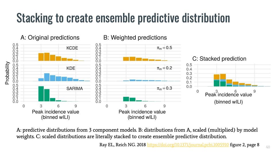
Stacking to create ensemble predictive distribution
A: predictive distributions from 3 component models. B: distributions from A, scaled (multiplied) by model weights. C: scaled distributions are literally stacked to create ensemble predictive distribution. Ray EL, Reich NG. 2018 https://doi.org/10.1371/journal.pcbi.1005910 figure 2, page 8
Presenter notes
Ray EL, Reich NG. Prediction of infectious disease epidemics via weighted density ensembles. PLoS Computational Biology. 2018 Feb 20;14(2):e1005910. https://doi.org/10.1371/journal.pcbi.1005910 figure 2, page 8
Slide 41What are ensemble methods? Super Learner?
We saw 2 kinds of tree ensembles:
Random forests use bagging—equal weight to several models
AdaBoost uses boosting—extra weight to poorly performing models to improve learning
These methods, and a third, combine any set of models—even different architectures
Stacking constructs a weighted average of component models; weights are learned
Super Learner is a popular, theory-supported stacking routine with good properties
Slide 42Examples of ensemble methods (2)
Petersen ML et al. Super learner analysis of electronic adherence data improves viral prediction and may provide strategies for selective HIV RNA monitoring. 2015. https://doi.org/10.1097/QAI.0000000000000548 [CDC/ATSDR][Open Access]
Super Learner (5 component models) to classify viral failure among 1478 adults on ART and monitored for adherence; cut ≥25% tests and still maintain Se ≥ 95%
Herrera R et al. Estimating the causal impact of proximity to gold and copper mines on respiratory diseases in Chilean children: An application of targeted maximum likelihood estimation. 2018. https://doi.org/10.3390/ijerph15010039 [Open Access]
Super learner: causal attributable risk for asthma or allergic rhinoconjunctivitis; living away from mine would decrease conjunctivitis risk by 4.7 percentage points
Abbreviations: ART = antiretroviral therapy; ATSDR = Agency for Toxic Substances and Disease Registry; CDC = Centers for Disease Control and Prevention; HIV = human immunodeficiency virus; ML = machine learning; RNA = ribonucleic acid.
Slide 43Further remarks on ensemble methods
Influenza season forecasts from distinct models can be combined as an ensemble
Influenza Division’s FluSight uses unweighted average
Some researchers propose stacking with a dynamic weighted average:
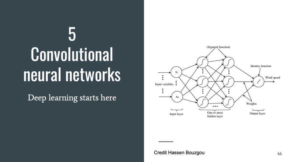
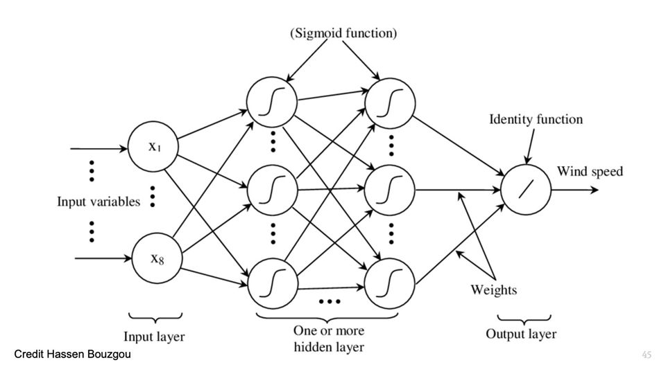
directed graph representing a feedforward neural network with an input layer, one or more hidden layers, and an output layer; nodes transform inputs; weight combine inputs to next layer
Slide 45Architecture of a multilayer perceptron neural network
Credit Hassen Bouzgou
Description
directed graph representing a feedforward neural network with an input layer, one or more hidden layers, and an output layer; nodes transform inputs; weight combine inputs to next layer
CNNs on 3 microscopy tasks in Uganda: malaria in thick blood smears, TB in sputum, hookworm eggs in stool. AUROC ≥ 0.99, way better than traditional medical imaging techniques.
Fine-tuned pretrained CNN to predict cluster-level nighttime light intensities from daytime satellite imagery; ridge regression to estimate cluster-level expenditures or assets; sidestepped need for labeled data
Abbreviations: AUROC = area under the relative operating characteristic (ROC) curve; CNN = convolutional neural network; TB = tuberculosis.
Slide 47What are neural networks? (and perceptrons?)
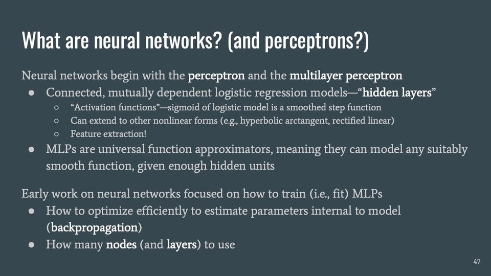
Neural networks begin with the perceptron and the multilayer perceptron
“Activation functions”—sigmoid of logistic model is a smoothed step function
Can extend to other nonlinear forms (e.g., hyperbolic arctangent, rectified linear)
Feature extraction!
MLPs are universal function approximators, meaning they can model any suitably smooth function, given enough hidden units
Early work on neural networks focused on how to train (i.e., fit) MLPs
How to optimize efficiently to estimate parameters internal to model (backpropagation)
How many nodes (and layers) to use
Abbreviations: MLP = multilayer perceptron.
Slide 48What are convolutional neural networks?
Convolutional neural networks’ hidden units build in more dependency (“shared weights”) across nodes, to reuse/share information (filter) across the network, which can reduce the number of parameters compared to MLPs
Typically trained using stochastic gradient descent (cf. GPUs)
Data might be augmented by distortions of inputs (rotate, reflect, etc.)
Each pass over the data is an epoch
Regularize using “dropout”
With conditional random fields, how USPS parses handwritten ZIP Codes
In contrast to previous computer vision tasks, CNNs can learn without user-constructed features
Abbreviations: CNN = convolutional neural network; GPUs = graphics processing units; MLP = multilayer perceptron; USPS = United States Postal Service; ZIP = Zone Improvement Plan (in "ZIP Codes").
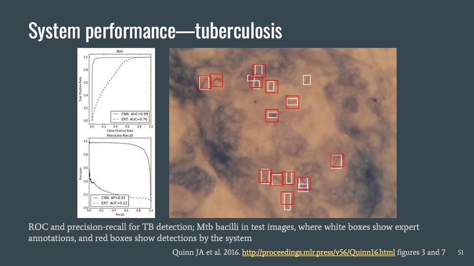
ROC and precision-recall for TB detection; Mtb bacilli in test images, where white boxes show expert annotations, and red boxes show detections by the system Quinn JA et al. 2016. http://proceedings.mlr.press/v56/Quinn16.html figures 3 and 7
Presenter notes
ROC and precision-recall for TB detection, showing Area Under Curve (AUC) and Average Precision (AP) Detected tuberculosis bacilli in test images; white boxes show expert annotations on pathogen locations; red boxes show detections by the system. Quinn JA et al. 2016. http://proceedings.mlr.press/v56/Quinn16.html
Abbreviations: AP = average precision; AUC = area under the curve; Mtb = Mycobacterium tuberculosis (the bacterium that causes TB); ROC = relative operating characteristic; TB = tuberculosis.
Slide 52Examples of convolutional neural networks (2)
CNNs on 3 microscopy tasks in Uganda: malaria in thick blood smears, TB in sputum, hookworm eggs in stool. AUROC ≥ 0.99, way better than traditional medical imaging techniques.
Fine-tuned pretrained CNN to predict cluster-level nighttime light intensities from daytime satellite imagery; ridge regression to estimate cluster-level expenditures or assets; sidestepped need for labeled data
Abbreviations: AUROC = area under the relative operating characteristic (ROC) curve; CNN = convolutional neural network; TB = tuberculosis.
Slide 53Further remarks on convolutional neural networks
Multilayer perceptrons were a popular machine learning solution in the 1980s.
SVMs took over for a while.
Then backpropagation (and, later, GPUs) led to deep learning.
While MLP is a universal function approximator, CNN approximately resolves into component objects (manifolds) that are complicated representations of features
Other applications of CNN, beyond static images:
NLP: parsing, search query, sentence modeling
Drug discovery by predicting interaction between molecules and proteins (treatments for Ebola virus and multiple sclerosis)
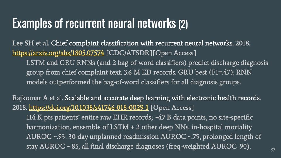
Lee SH et al. Chief complaint classification with recurrent neural networks. 2018. https://arxiv.org/abs/1805.07574 [CDC/ATSDR][Open Access]
LSTM and GRU RNNs (and 2 bag-of-word classifiers) predict discharge diagnosis group from chief complaint text. 3.6 M ED records. GRU best (F1=.47); RNN models outperformed the bag-of-word classifiers for all diagnosis groups.
114 K pts patients’ entire raw EHR records; ~47 B data points, no site-specific harmonization. ensemble of LSTM + 2 other deep NNs. in-hospital mortality AUROC ~.93, 30-day unplanned readmission AUROC ~.75, prolonged length of stay AUROC ~.85, all final discharge diagnoses (freq-weighted AUROC .90).
Abbreviations: ATSDR = Agency for Toxic Substances and Disease Registry; AUROC = area under the relative operating characteristic (ROC) curve; CDC = Centers for Disease Control and Prevention; ED = emergency department; EHR = electronic health record; GRU = gated recurrent unit; LSTM = long short-term memory (a kind of recurrent neural network); NN = neural network; RNN = recurrent neural network.
Slide 56What are recurrent neural networks?
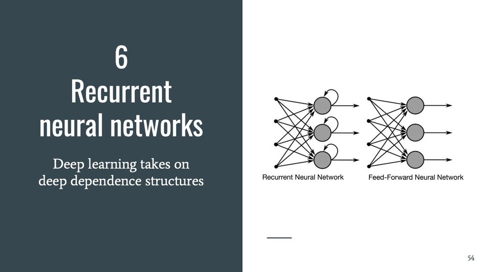
MLPs and CNNs are feedforward networks: dependencies go in 1 direction; they cannot represent temporal dynamic behavior
Enter recurrent neural networks (RNNs)
Back-connections maintain (“remember”) previous states during updates, enabling sequence prediction
Long short-term memory (LSTM) stabilizes by preventing certain kinds of errors (using a “forget gate”), thus improving ability to handle sequential data
Gated recurrent unit (GRU) simplifies LSTM (but doesn’t do all the same tasks)
Bi-directional RNNs process sequential input in forward and backward
Lee SH et al. Chief complaint classification with recurrent neural networks. 2018. https://arxiv.org/abs/1805.07574 [CDC/ATSDR][Open Access]
LSTM and GRU RNNs (and 2 bag-of-word classifiers) predict discharge diagnosis group from chief complaint text. 3.6 M ED records. GRU best (F1=.47); RNN models outperformed the bag-of-word classifiers for all diagnosis groups.
114 K pts patients’ entire raw EHR records; ~47 B data points, no site-specific harmonization. ensemble of LSTM + 2 other deep NNs. in-hospital mortality AUROC ~.93, 30-day unplanned readmission AUROC ~.75, prolonged length of stay AUROC ~.85, all final discharge diagnoses (freq-weighted AUROC .90).
Abbreviations: ATSDR = Agency for Toxic Substances and Disease Registry; AUROC = area under the relative operating characteristic (ROC) curve; CDC = Centers for Disease Control and Prevention; ED = emergency department; EHR = electronic health record; GRU = gated recurrent unit; LSTM = long short-term memory (a kind of recurrent neural network); NN = neural network; RNN = recurrent neural network.
Slide 58Further remarks on recurrent neural networks
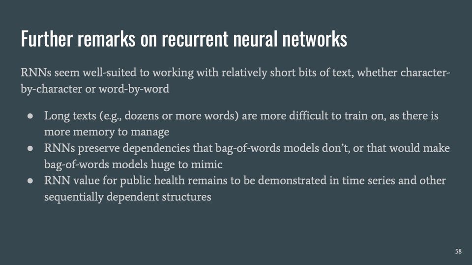
RNNs seem well-suited to working with relatively short bits of text, whether character-by-character or word-by-word
Long texts (e.g., dozens or more words) are more difficult to train on, as there is more memory to manage
RNNs preserve dependencies that bag-of-words models don’t, or that would make bag-of-words models huge to mimic
RNN value for public health remains to be demonstrated in time series and other sequentially dependent structures
Abbreviations: RNN = recurrent neural network.
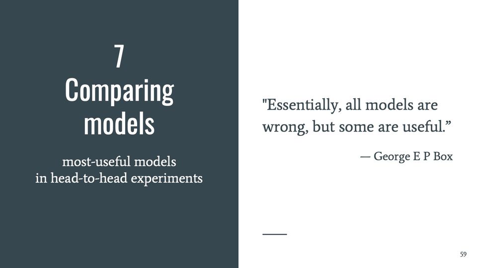
Slide 597. Comparing models
most-useful models in head-to-head experiments
"Essentially, all models are wrong, but some are useful.”
— George E P Box
Slide 60Examples of experiments comparing models (1)
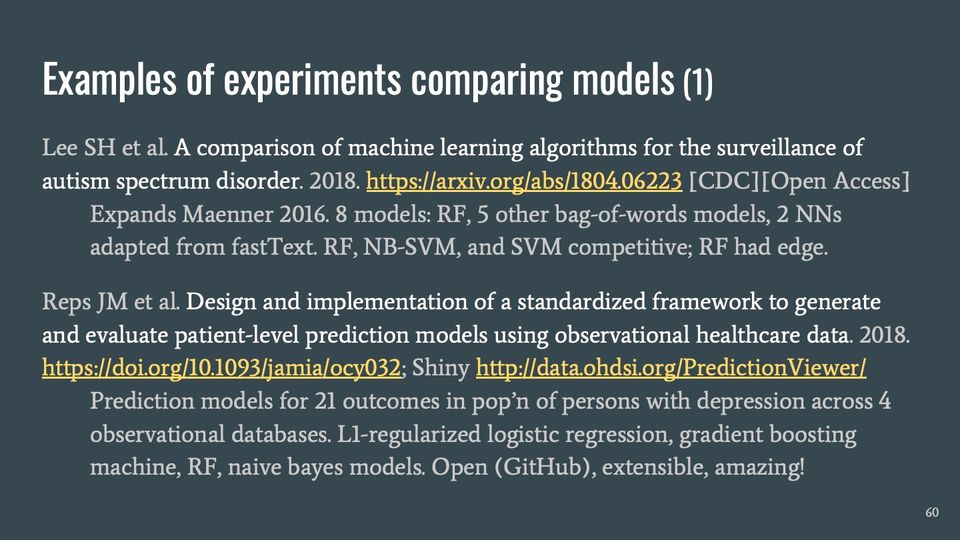
Lee SH et al. A comparison of machine learning algorithms for the surveillance of autism spectrum disorder. 2018. https://arxiv.org/abs/1804.06223 [CDC][Open Access]
Expands Maenner 2016. 8 models: RF, 5 other bag-of-words models, 2 NNs adapted from fastText. RF, NB-SVM, and SVM competitive; RF had edge.
Prediction models for 21 outcomes in pop’n of persons with depression across 4 observational databases. L1-regularized logistic regression, gradient boosting machine, RF, naive bayes models. Open (GitHub), extensible, amazing!
Abbreviations: CDC = Centers for Disease Control and Prevention; NB = naive Bayes; NN = neural network; OHDSI = Observational Health Data Sciences and Informatics; RF = random forest; SVM = support vector machine.
Slide 61What goes into machine learning experiments?
We have conventional tools for comparing statistical models with similar architecture, such as information criteria (e.g., Akaike, Bayes/Schwarz)
Compare machine-learned on empirical performance, typically by cross-validation
Common performance measures
F1, harmonic mean of sensitivity and PPV, insensitive to true negatives
AUROC, function of sensitivity and specificity
Calibration
Ensure that pseudorandomness is managed properly (k folds, train/val/test)
Over multiple datasets: Wilcoxon signed-rank, Friedman, multiplicity adjustments and post hoc corrections
Abbreviations: AUROC = area under the relative operating characteristic (ROC) curve; PPV = positive predictive value.
Slide 62Examples of experiments comparing models (2)
Lee SH et al. A comparison of machine learning algorithms for the surveillance of autism spectrum disorder. 2018. https://arxiv.org/abs/1804.06223 [CDC][Open Access]
Expands Maenner 2016. 8 models: RF, 5 other bag-of-words models, 2 NNs adapted from fastText. RF, NB-SVM, and SVM competitive; RF had edge.
Prediction models for 21 outcomes in pop’n of persons with depression across 4 observational databases. L1-regularized logistic regression, gradient boosting machine, RF, naive bayes models. Open (GitHub), extensible, amazing!
Abbreviations: CDC = Centers for Disease Control and Prevention; NB = naive Bayes; NN = neural network; OHDSI = Observational Health Data Sciences and Informatics; RF = random forest; SVM = support vector machine.
Slide 63Further remarks on machine learning experiments
Machine learning experiments should be reproducible
Lee 2018 Python code is publicly available (though the data are privileged)
Reps 2018 is an open-source example (R and Python components) of a reproducible, extensible workflow for machine learning experiments (though the data in the manuscript are privileged)
Slide 648. Machine learning isn’t everything (and other thoughts)
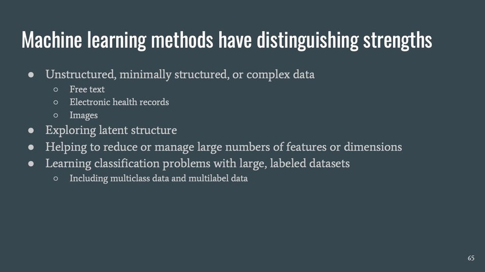
Slide 65Machine learning methods have distinguishing strengths
Unstructured, minimally structured, or complex data
Free text
Electronic health records
Images
Exploring latent structure
Helping to reduce or manage large numbers of features or dimensions
Learning classification problems with large, labeled datasets
Including multiclass data and multilabel data
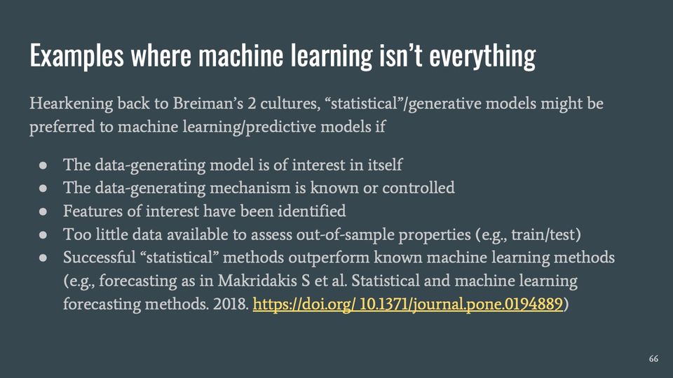
Slide 66Examples where machine learning isn’t everything
Hearkening back to Breiman’s 2 cultures, “statistical”/generative models might be preferred to machine learning/predictive models if
The data-generating model is of interest in itself
The data-generating mechanism is known or controlled
Features of interest have been identified
Too little data available to assess out-of-sample properties (e.g., train/test)
Successful “statistical” methods outperform known machine learning methods (e.g., forecasting as in Makridakis S et al. Statistical and machine learning forecasting methods. 2018. https://doi.org/ 10.1371/journal.pone.0194889)
Presenter notes
Makridakis S et al. Statistical and machine learning forecasting methods. 2018. https://doi.org/ 10.1371/journal.pone.0194889
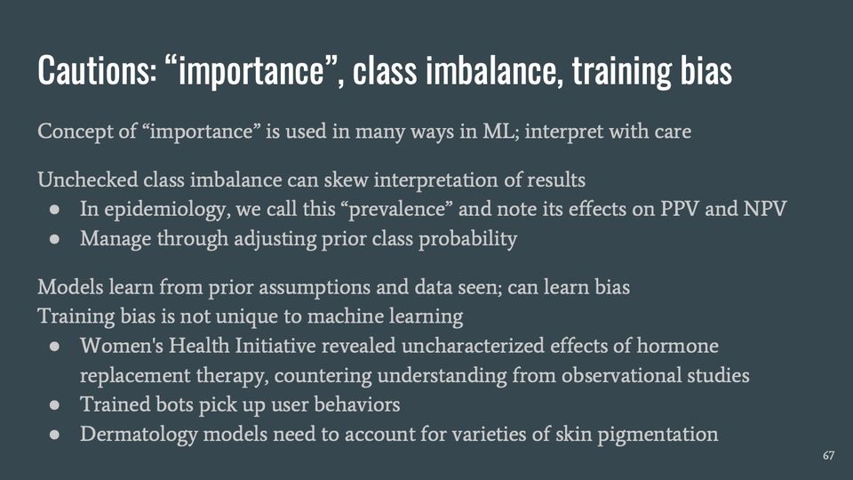
Slide 67Cautions: “importance”, class imbalance, training bias
Concept of “importance” is used in many ways in ML; interpret with care
Unchecked class imbalance can skew interpretation of results
In epidemiology, we call this “prevalence” and note its effects on PPV and NPV
Manage through adjusting prior class probability
Models learn from prior assumptions and data seen; can learn bias
Training bias is not unique to machine learning
Women's Health Initiative revealed uncharacterized effects of hormone replacement therapy, countering understanding from observational studies
Trained bots pick up user behaviors
Dermatology models need to account for varieties of skin pigmentation
Presenter notes
example from conventional statistical approaches: add or remove features (such as interaction terms); increase or decrease model complexity (knots in or degree of a spline) Adamson AS, Smith A. Machine learning and health care disparities in dermatology. 2018. https://doi.org/10.1001/jamadermatol.2018.2348
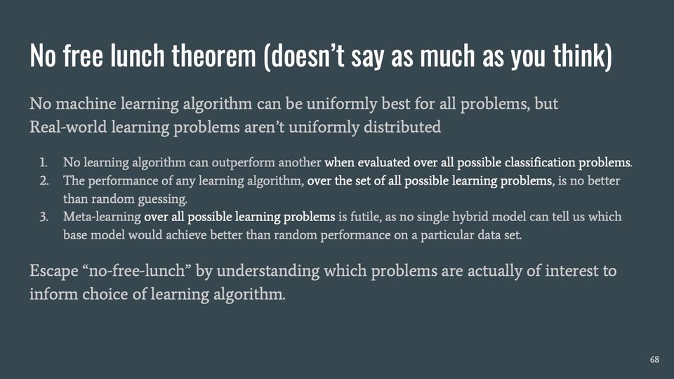
No learning algorithm can outperform another when evaluated over all possible classification problems.
The performance of any learning algorithm, over the set of all possible learning problems, is no better than random guessing.
Meta-learning over all possible learning problems is futile, as no single hybrid model can tell us which base model would achieve better than random performance on a particular data set.
Escape “no-free-lunch” by understanding which problems are actually of interest to inform choice of learning algorithm.
Presenter notes
quoted and paraphrased from Flach 2012, pp 20, 340-341
Slide 699. Wrapping up
not a machine learning task, per se
Presenter notes
[redacted: intranet URL] [redacted: intranet URL]
Slide 70Whirlwind tour of 7 kinds of applications—a primer
Tasks that look like regression
Support vector machines
Random forests (and other tree-based methods)
Combining different models
Convolutional neural networks
Recurrent neural networks
Comparing models
Machine learning has been applied to an increasing variety of public health problems. The set of interesting questions expands with more awareness of methods and more kinds of data.
Slide 71Fin
Material will be available, including this talk, annotated bibliography, discussion boards, sample code SharePoint: [redacted: intranet URL] GitLab: [redacted: intranet URL] Data Hub: Chad Heilig, PhD • [redacted: email address] Scott Lee, PhD • [redacted: email address] CSELS Machine Learning • [redacted: email address] CSELS Data Hub Webinar, 2018-11-19
Description
Text in the picture
data hub
Presenter notes
add SharePoint and Git URLs
Abbreviations: CSELS = Center for Surveillance, Epidemiology, and Laboratory Services (CDC); URLs = uniform resource locators (web addresses).
https://xkcd.com/2048/ Curve-Fitting Methods and the messages they send [In a single frame twelve scatter plots with unlabeled x- and y-axes are shown. Each plot consists of the same data-set of approximately thirty points located all over the plot but slightly more distributed around the diagonal. Every plot shows in red a different fitting method which is labeled on top in gray.] [The first plot shows a line starting at the left bottom above the x-axis rising towards the points to the right.] Linear "Hey, I did a regression." [The second plot shows a curve falling slightly down and then rising up to the right.] Quadratic "I wanted a curved line, so I made one with math." [At the third plot the curve starts near the left bottom and increases more and more less to the right.] Logarithmic "Look, it's tapering off!" [The fourth plot shows a curve starting near the left bottom and increases more and more steeper towards the right.] Exponential "Look, it's growing uncontrollably!" [The fifth plot uses a fitting to match many points. It starts at the left bottom, increases, then decreases, then rapidly increasing again, and finally reaching a plateau.] LOESS "I'm sophisticated, not like those bumbling polynomial people." [The sixth plot simply shows a line above but parallel to the x-axis.] Linear, no slope "I'm making a scatter plot but I don't want to." [At plot #7 starts at a plateau above the x-axis, then increases, and finally reaches a higher plateau.] Logistic "I need to connect these two lines, but my first idea didn't have enough Math." [Plot #8 shows two red lines embedding most points and the area between is painted as a red shadow.] Confidence interval "Listen, science is hard. But I'm a serious person doing my best." [Plot #9 shows two not connected lines, one at the lower left half, and one higher at the right. Both have smaller curved lines in light red above and below.] Piecewise "I have a theory, and this is the only data I could find." [The plot at the left bottom shows a line connecting all points from left to right, resulting in a curve going many times up and down.] Connecting lines "I clicked 'Smooth Lines' in Excel." [The next to last plot shows a echelon form, connecting a few real and some imaginary points.] Ad-Hoc filter "I had an idea for how to clean up the data. What do you think?" [The last plot shows a wave with increasing peak values. Finally the plot of the wave is continued beyond the x- and y-axis borders.] House of Cards "As you can see, this model smoothly fits the- wait no no don't extend it AAAAAA!!"
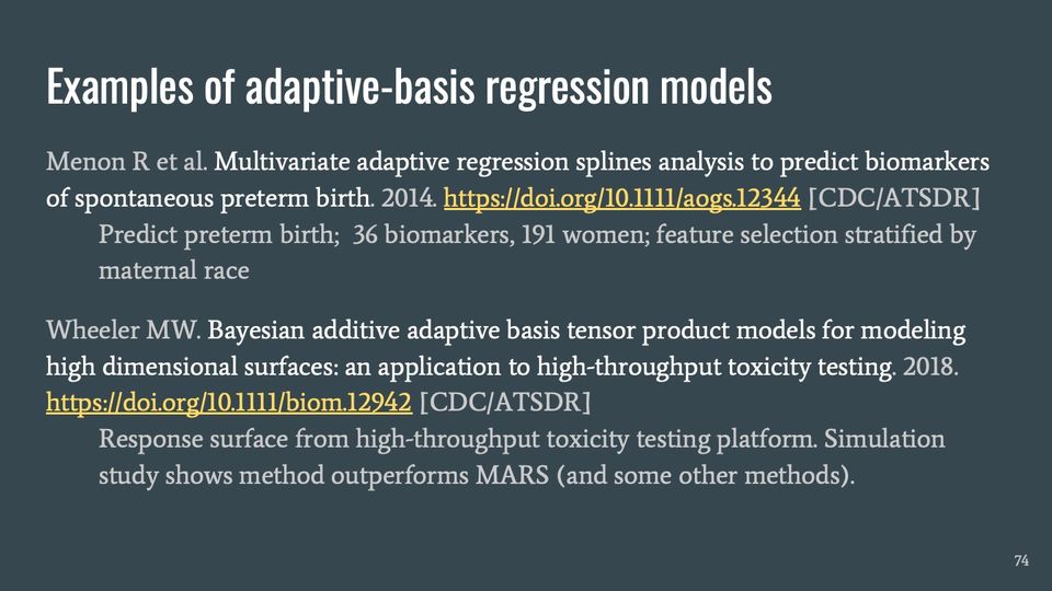
Slide 74Examples of adaptive-basis regression models
Menon R et al. Multivariate adaptive regression splines analysis to predict biomarkers of spontaneous preterm birth. 2014. https://doi.org/10.1111/aogs.12344 [CDC/ATSDR]
Wheeler MW. Bayesian additive adaptive basis tensor product models for modeling high dimensional surfaces: an application to high-throughput toxicity testing. 2018. https://doi.org/10.1111/biom.12942 [CDC/ATSDR]
Response surface from high-throughput toxicity testing platform. Simulation study shows method outperforms MARS (and some other methods).
Abbreviations: ATSDR = Agency for Toxic Substances and Disease Registry; CDC = Centers for Disease Control and Prevention; MARS = multivariate adaptive regression splines.
Slide 75Other notable examples of ML for public health
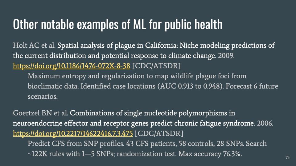
Holt AC et al. Spatial analysis of plague in California: Niche modeling predictions of the current distribution and potential response to climate change. 2009. https://doi.org/10.1186/1476-072X-8-38 [CDC/ATSDR]
Maximum entropy and regularization to map wildlife plague foci from bioclimatic data. Identified case locations (AUC 0.913 to 0.948). Forecast 6 future scenarios.
Goertzel BN et al. Combinations of single nucleotide polymorphisms in neuroendocrine effector and receptor genes predict chronic fatigue syndrome. 2006. https://doi.org/10.2217/14622416.7.3.475 [CDC/ATSDR]
Predict CFS from SNP profiles. 43 CFS patients, 58 controls, 28 SNPs. Search ~122K rules with 1—5 SNPs; randomization test. Max accuracy 76.3%.
Presenter notes
‘most important SNPs’ not identical to ‘most differentiating SNPs’
Abbreviations: ATSDR = Agency for Toxic Substances and Disease Registry; AUC = area under the curve; CDC = Centers for Disease Control and Prevention; CFS = chronic fatigue syndrome; ML = machine learning; SNP = single-nucleotide polymorphism.
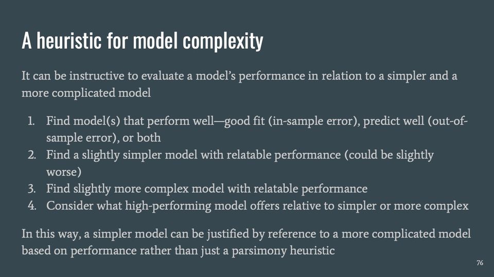
Slide 76A heuristic for model complexity
It can be instructive to evaluate a model’s performance in relation to a simpler and a more complicated model
Find model(s) that perform well—good fit (in-sample error), predict well (out-of-sample error), or both
Find a slightly simpler model with relatable performance (could be slightly worse)
Find slightly more complex model with relatable performance
Consider what high-performing model offers relative to simpler or more complex
In this way, a simpler model can be justified by reference to a more complicated model based on performance rather than just a parsimony heuristic
Presenter notes
example from conventional statistical approaches: add or remove features (such as interaction terms); increase or decrease model complexity (knots in or degree of a spline)
Slide 77Resources
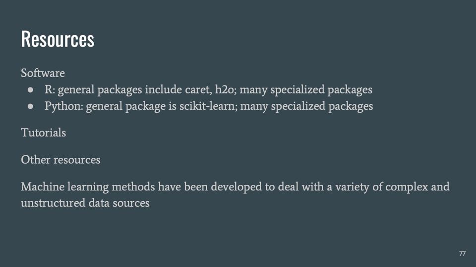
Software
R: general packages include caret, h2o; many specialized packages
Python: general package is scikit-learn; many specialized packages
Tutorials
Other resources
Machine learning methods have been developed to deal with a variety of complex and unstructured data sources
Abbreviations
AIMIE = AI in Medicine: Inclusion & Equity symposium; AP = average precision; ART = antiretroviral therapy; ASD = autism spectrum disorder; ATSDR = Agency for Toxic Substances and Disease Registry; AUC = area under the curve; AUROC = area under the relative operating characteristic (ROC) curve; CART = classification and regression trees; CDC = Centers for Disease Control and Prevention; CFS = chronic fatigue syndrome; CHSI = Community Health Status Indicators; CMIM = conditional mutual information maximization (a feature-selection method); CNN = convolutional neural network; CpG = CpG (cytosine–phosphate–guanine) site; CPR = Center for Preparedness and Response (CDC); CSELS = Center for Surveillance, Epidemiology, and Laboratory Services (CDC); DCPC = Division of Cancer Prevention and Control (CDC/NCCDPHP); DEO = Division of Emergency Operations (CDC); DHIS = Division of Health Informatics and Surveillance (CDC, in CSELS); DNA = deoxyribonucleic acid; DNPAO = Division of Nutrition, Physical Activity, and Obesity (CDC/NCCDPHP); DPHID = Division of Public Health Information Dissemination (CDC/CSELS); ED = emergency department; EHR = electronic health record; GPUs = graphics processing units; GRU = gated recurrent unit; HHS = Department of Health and Human Services; HIV = human immunodeficiency virus; IBM = individual-based model; ICU = intensive care unit; ISBN = International Standard Book Number; KE = Kenya; LOESS = locally estimated scatterplot smoothing; LSTM = long short-term memory (a kind of recurrent neural network); MARS = multivariate adaptive regression splines; ML = machine learning; MLP = multilayer perceptron; Mtb = Mycobacterium tuberculosis (the bacterium that causes TB); NB = naive Bayes; NCBDDD = National Center on Birth Defects and Developmental Disabilities (CDC); NCCDPHP = National Center for Chronic Disease Prevention and Health Promotion (CDC); NCHS = National Center for Health Statistics (CDC); NCIPC = National Center for Injury Prevention and Control (CDC); NCIRD = National Center for Immunization and Respiratory Diseases (CDC); NIOSH = National Institute for Occupational Safety and Health (CDC); NLP = natural language processing; NN = neural network; NPV = negative predictive value; OHDSI = Observational Health Data Sciences and Informatics; OPHSS = Office of Public Health Scientific Services (CDC); PAF = population attributable fraction; PCA = principal component analysis; PPV = positive predictive value; RF = random forest; RNA = ribonucleic acid; RNN = recurrent neural network; ROC = relative operating characteristic; SNP = single-nucleotide polymorphism; SVM = support vector machine; TB = tuberculosis; URLs = uniform resource locators (web addresses); USPS = United States Postal Service; ZIP = Zone Improvement Plan (in "ZIP Codes").
References, compiled for this page
Full citations, with current links, for selected references and related works.
Lee SH, Levin D, Finley PD, Heilig CM. Chief complaint classification with recurrent neural networks. Journal of Biomedical Informatics. 2019-05; 93: 103158. (slides55, 57)Elsewhere on the web (opens in a new tab)
Lee SH, Maenner MJ, Heilig CM. A comparison of machine learning algorithms for the surveillance of autism spectrum disorder. PLOS ONE. 2019-09-25; 14(9): e0222907. (slides60, 62)Elsewhere on the web (opens in a new tab)
Maenner MJ, Yeargin-Allsopp M, Van Naarden Braun K, Christensen DL, Schieve LA. Development of a machine learning algorithm for the surveillance of autism spectrum disorder. PLoS ONE. 2016-12-21; 11(12): e0168224. (slides29, 35)Elsewhere on the web (opens in a new tab)