Statistical decisions: the elements of testing hypotheses
This rendering was constructed from an original PowerPoint presentation. Corrections of original text are indicated as “[corrected: X]”, redactions as “[redacted: X]”, and names withheld as “[generalized: X]”. Handouts and other auxiliary sources mentioned in the presentations are not available. The content of each presentation was believed to be correct and valid at the time of the presentation. This content, including references and links within the slides, has not been checked or updated when preparing this site. This rendering was facilitated by Anthropic Claude agentic tools for automated text extraction through computer vision and for assistance with compiling the completed sets.
Setting: Statistical decisions: the elements of testing hypotheses, 2002-07-11. CDC’s Epidemic Intelligence Service (EIS) summer course, 70+ incoming postdoctoral fellows, mostly physicians and epidemiologists.
They understood less after my lecture than before it. And not in some appreciate-what-you-have-yet-to-learn kind of way. Among respondents, 40% said that they had basic, little, or no knowledge or skill in the subject matter before my seminar. After the seminar, that number climbed to 57% – a net loss of 17%.
I had led a 3-hour seminar titled “Statistical decisions: the elements of testing hypotheses” for CDC’s EIS summer course, populated by several dozen incoming postdoctoral fellows – physicians and epidemiologists and other learners. I’d poured my heart into a session motivated by intuition and followed by practical rigor.
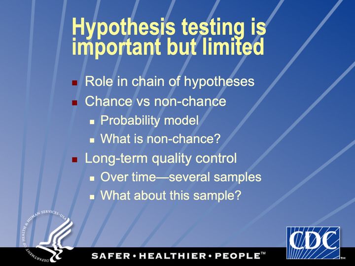
- Thesis: A proper hypothesis test serves 1 function: to distinguish chance from nonchance influences, with long-run control of the error rate. “Nothing less / Equally important, nothing more.” Slide 2
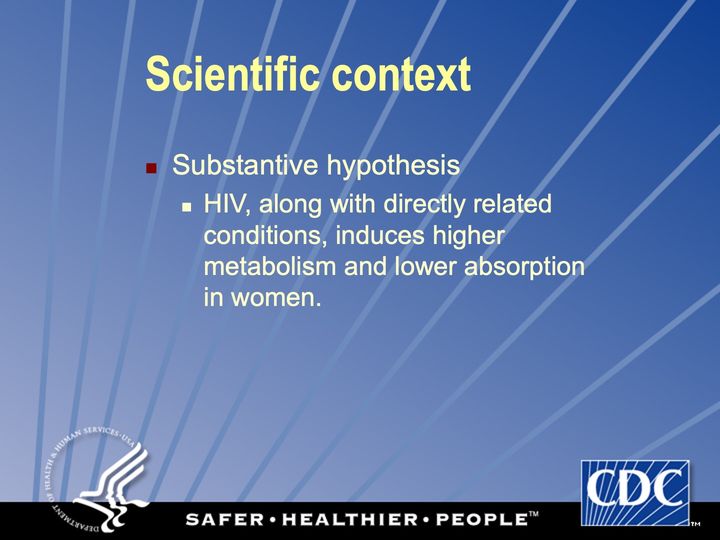
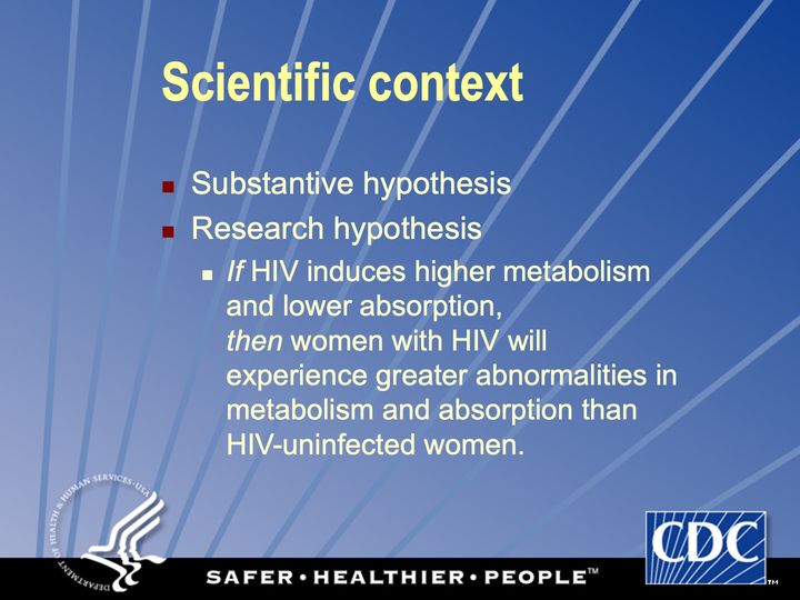
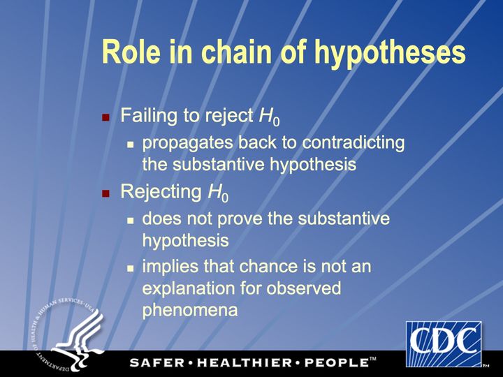
- Part 1. A running example. A chain of hypotheses (substantive → research → experimental → statistical) asks whether women with HIV have lower mean body mass index, using data from the HIV Epidemiology Research (HER) Study.
- Part 2. Common tests on HER Study data, including z, t, proportions, Pearson, Fisher, McNemar, Wilcoxon.
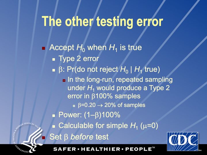
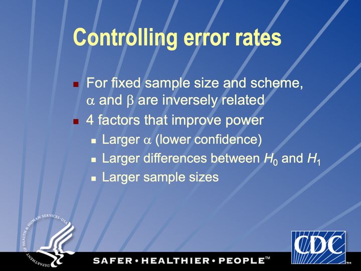
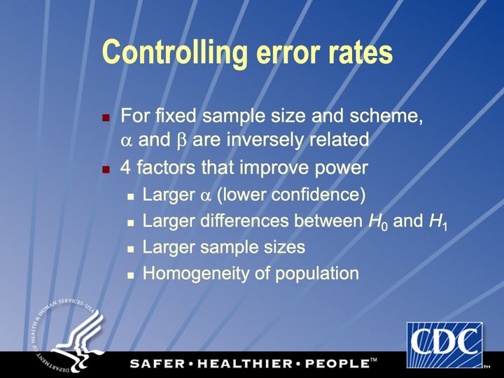
- Part 3. Practical and ethical limits: P’s “one proper role” is a personal α; small P ≠ important; the ethics of H_0, α and β; 4 ways to raise power; decisions are not evidence.
- Part 4. “A personal word”, now lost to history.
Join me in my supervillain origin story, through the vicissitudes of selected evaluations:
- What parts of the session need improvement? “all of it” • “entirely overshot or misjudged the audience”.
- What did the instructor do best? “‘personal’ take at end” • “emphasize caveats, care” • “good intentions” • “he was very patient with us” • “knew what he was talking about” • “appears to enjoy material”.
- Comments: “great stats review - very hard since this amount of material would normally be covered in a whole semester” • “basically took concepts that I thought I understood and managed to thoroughly confuse me”.
In fairness, I had quoted Alan Greenspan: “If I have made myself clear, you must have misunderstood me.” I threw this in too, with apologies: “All we are saying is give chance some Ps”. Slide 53
This polarizing presentation is an important part of my intellectual history. Since then, I have turned my teaching and mentoring ways to the cause of good rather than evil. I have won plaudits from learners and the EIS program itself. And I have envisioned a whole progressive culture for doing good things with data.
Works referred to
- Heilig (2025)On this site (opens in a new tab)
- Paramsothy et al. (2004)Elsewhere on the web (opens in a new tab)
- Phelps et al. (2001)Elsewhere on the web (opens in a new tab)
- Tohill et al. (2007)Elsewhere on the web (opens in a new tab)
Full references: this page · whole site, by domain (opens in a new tab) · whole site, by type of work (opens in a new tab)
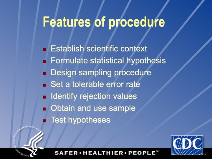
Text in the picture
DEPARTMENT OF HEALTH & HUMAN SERVICES • USA
CDC
SAFER • HEALTHIER • PEOPLE™
Abbreviations: CDC = Centers for Disease Control and Prevention; HHS = Department of Health and Human Services; USA = United States of America.
Emphasize intuition over derivation, practicality over theory, interpretation over calculation
Abbreviations: BMI = body mass index (kg/m²); HIV = human immunodeficiency virus.
Define BMI: mass in kilograms divided by height in meters, squared.
Abbreviations: BMI = body mass index (kg/m²); HIV = human immunodeficiency virus.
Abbreviations: HIV = human immunodeficiency virus.
Abbreviations: HIV = human immunodeficiency virus.
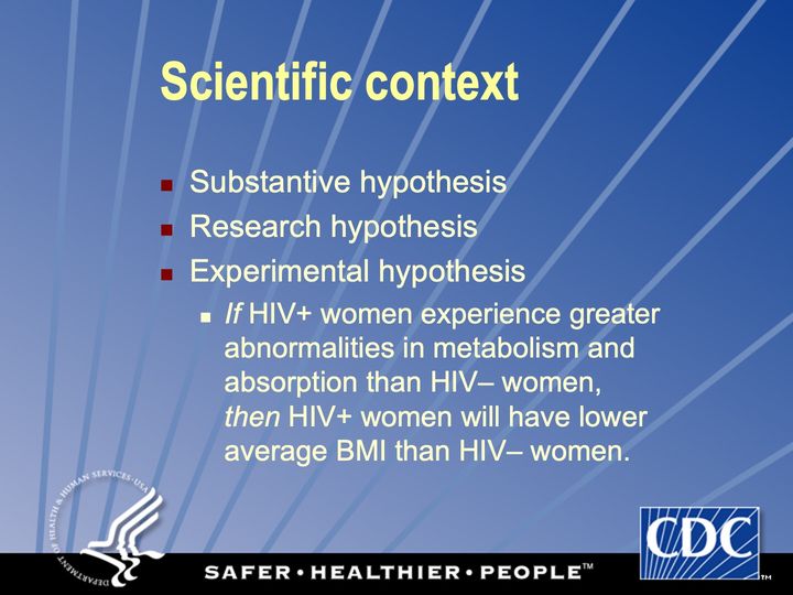
Abbreviations: BMI = body mass index (kg/m²); HIV = human immunodeficiency virus; HIV+ = HIV-positive.
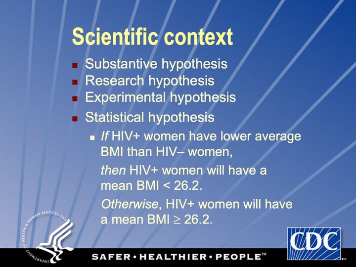
Suppose the population average BMI for US women is 26.2.
Abbreviations: BMI = body mass index (kg/m²); HIV = human immunodeficiency virus; HIV+ = HIV-positive; US = United States.
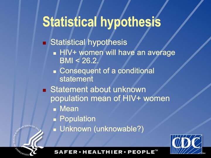
Abbreviations: BMI = body mass index (kg/m²); HIV+ = HIV-positive.
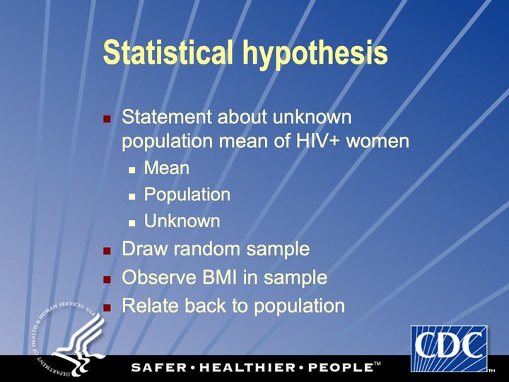
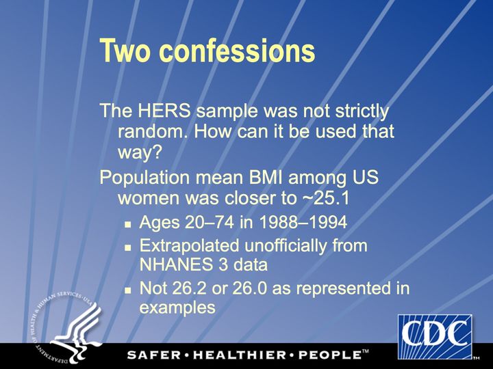
This sample is not really random
Abbreviations: BMI = body mass index (kg/m²); HIV+ = HIV-positive.
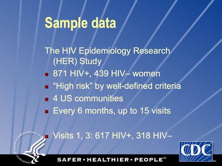
A sample of US women with HIV
Abbreviations: HER/HERS = HIV Epidemiology Research (HER) Study; HIV = human immunodeficiency virus; HIV+ = HIV-positive; US = United States.
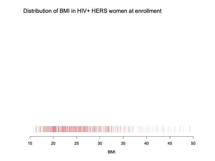
- Panels
- 1
- Elements
- A rug of thin vertical red tick marks in a single row near the bottom depicts individual BMI values; overlapping ticks appear darker
- Horizontal
- BMI, 15 to 50; ticks extend from about 16 to about 49
- Vertical
- No scale; the ticks occupy a narrow strip just above the axis, and the space above them, is empty
- Visible pattern
- The ticks are densest and darkest from about 18 to about 28, and they thin out from about 28 to about 37 and then become sparse.
Text in the picture
Distribution of BMI in HIV+ HERS women at enrollment
Abbreviations: BMI = body mass index (kg/m²); HER/HERS = HIV Epidemiology Research (HER) Study; HIV+ = HIV-positive.
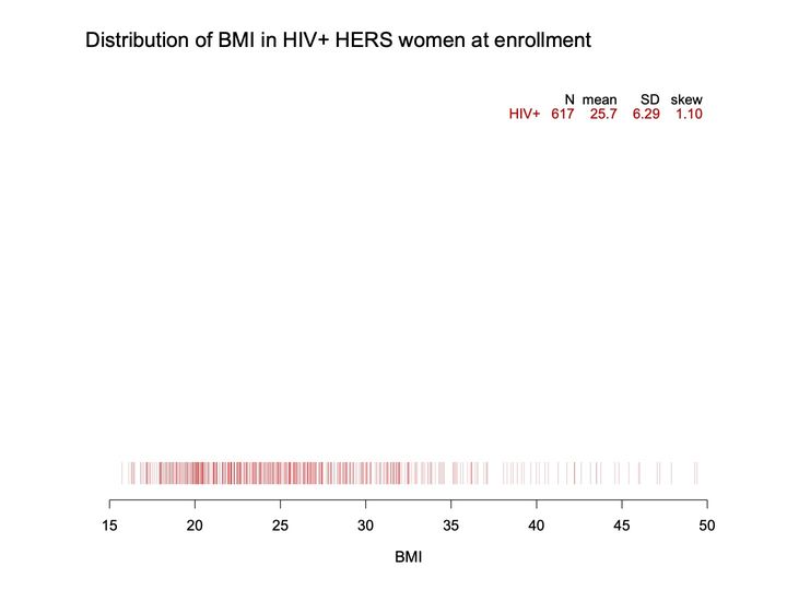
- Panels
- 1
- Elements
- A rug of thin vertical red tick marks in a single row near the bottom depicts individual BMI values; a small table of summary statistics in red and black sits at upper right
- Horizontal
- BMI, 15 to 50; ticks extend from about 16 to about 49
- Vertical
- No scale; the ticks occupy a narrow strip just above the axis; the space above them is empty apart from the table
- Visible pattern
- The ticks are densest and darkest from about 18 to about 28, and they thin out from about 28 to about 37 and then become sparse.
Text in the picture
Distribution of BMI in HIV+ HERS women at enrollment
N mean SD skew
HIV+ 617 25.7 6.29 1.10
Abbreviations: BMI = body mass index (kg/m²); HER/HERS = HIV Epidemiology Research (HER) Study; HIV+ = HIV-positive; SD = standard deviation.
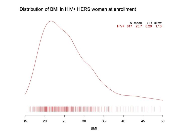
- Panels
- 1
- Elements
- 1 smoothed red curve depicts the shape of the BMI distribution, above a rug of thin vertical red tick marks depicting individual BMI values; a small table of summary statistics at upper right
- Horizontal
- BMI, 15 to 50; the curve spans the full extent, ticks from about 16 to about 49
- Vertical
- No scale or axis; the curve fills most of the plot height above the rug, peaking near the top
- Visible pattern
- The density curve peaks near BMI 22, then falls more gradually to about 40 and flattens into a long, low tail.
Text in the picture
Distribution of BMI in HIV+ HERS women at enrollment
N mean SD skew
HIV+ 617 25.7 6.29 1.10
Abbreviations: BMI = body mass index (kg/m²); HER/HERS = HIV Epidemiology Research (HER) Study; HIV+ = HIV-positive; SD = standard deviation.
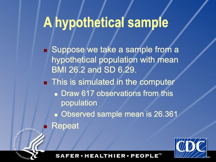
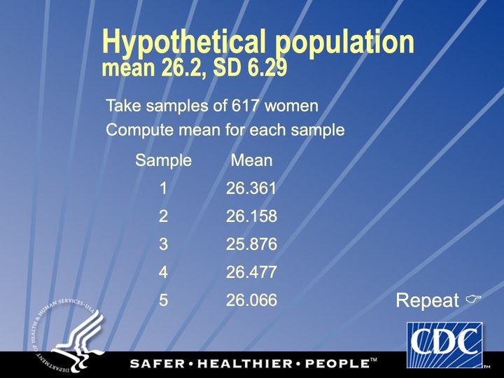
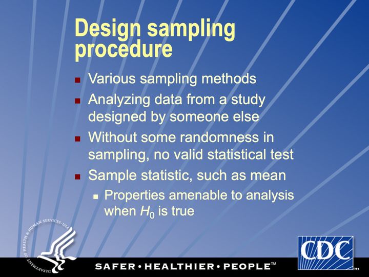
Abbreviations: BMI = body mass index (kg/m²); SD = standard deviation.
Because the HIV+ population mean is unknown
Abbreviations: HIV+ = HIV-positive.
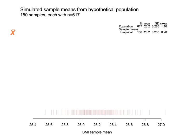
- Panels
- 1
- Elements
- 1 rug of thin pink vertical ticks depicts the simulated sample means; no curve
- Horizontal
- BMI sample mean, 25.4 to 27.0 in steps of 0.2; ticks run from about 25.55 to about 27.06, just past the end of the axis
- Vertical
- No vertical axis or scale; the ticks occupy a narrow band just above the horizontal axis, and the space above them is empty apart from the table
- Visible pattern
- The ticks crowd most densely between about 25.8 and 26.5 and thin out toward both ends. The right end trails further than the left, with widely spaced ticks from about 26.6 to just past 27.0, while the left end stops near 25.55 after a few scattered ticks.
Text in the picture
Simulated sample means from hypothetical population
150 samples, each with n=617
x̄
N mean SD skew
Population 617 26.2 6.286 1.10
Sample means
Empirical 150 26.2 0.260 0.20
Abbreviations: BMI = body mass index (kg/m²); SD = standard deviation.
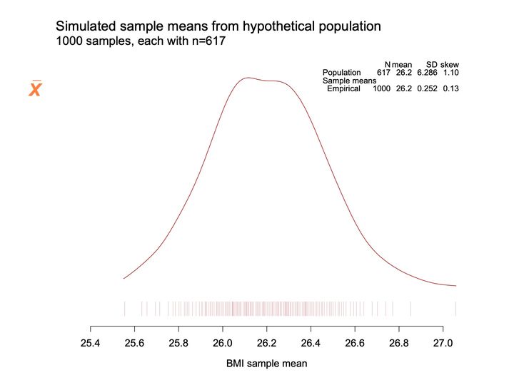
- Panels
- 1
- Elements
- 1 solid dark red density curve above a rug of thin pink vertical ticks; both depict simulated sample means
- Horizontal
- BMI sample mean, 25.4 to 27.0 in steps of 0.2; curve and ticks run from about 25.55 to about 27.06, just past the end of the axis
- Vertical
- No vertical axis or scale; the curve's peak reaches near the top of the plotting area
- Visible pattern
- The curve is single-humped with a broad, nearly flat top spanning about 26.1 to 26.3. It rises more steeply on the left, where it ends near 25.55, and falls more gradually on the right, trailing to about 27.06. The ticks beneath are densest between about 25.8 and 26.5 and sparse at both ends.
Text in the picture
Simulated sample means from hypothetical population
1000 samples, each with n=617
x̄
N mean SD skew
Population 617 26.2 6.286 1.10
Sample means
Empirical 1000 26.2 0.252 0.13
Abbreviations: BMI = body mass index (kg/m²); SD = standard deviation.
- Panels
- 1
- Elements
- 2 dark red density curves (1 solid, 1 dashed) above a rug of thin pink vertical ticks; both density curves and ticks depict sample means; a faint gray dashed vertical reference line
- Horizontal
- BMI sample mean, 25.4 to 27.0 in steps of 0.2; reference line at 26.2; the solid curve runs from about 25.55 to about 27.06, the dashed curve from about 25.3 to past 27.0, beyond both ends of the axis
- Vertical
- No vertical axis or scale; the dashed curve's peak reaches the top of the plotting area
- Visible pattern
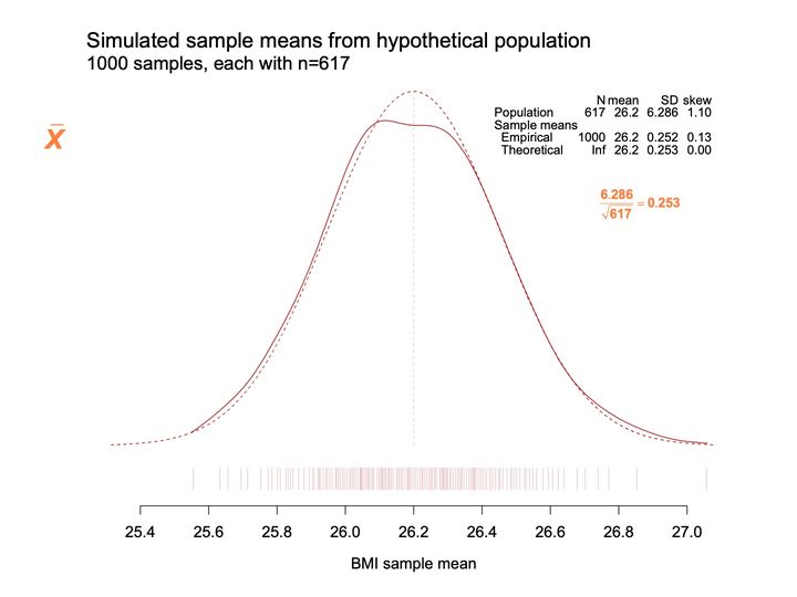
- The dashed curve is a smooth symmetric bell centered on the reference line at 26.2 and peaks above the solid curve. The solid curve follows it closely over most of the range: lower and flatter at the top, slightly outside it on the left flank, and slightly above it in the right tail from about 26.7 onward. The dashed curve extends past both ends of the solid curve.
Text in the picture
Simulated sample means from hypothetical population
1000 samples, each with n=617
x̄
N mean SD skew
Population 617 26.2 6.286 1.10
Sample means
Empirical 1000 26.2 0.252 0.13
Theoretical Inf 26.2 0.253 0.00
6.286 / √617 = 0.253
Be clear on SD and SE
Abbreviations: BMI = body mass index (kg/m²); SD = standard deviation; SE = standard error.
- Panels
- 1
- Elements
- 2 dark red density curves (1 solid, 1 dashed) above a rug of thin pink vertical ticks depict shifted sample means; a faint gray dashed vertical reference line
- Horizontal
- Labeled BMI sample mean, -0.8 to 0.8 in steps of 0.2; reference line at 0.0; ticks run from about -0.65 to about 0.86; the dashed curve extends past both ends of the axis
- Vertical
- No vertical axis or scale; the dashed curve's peak reaches the top of the plotting area
- Visible pattern
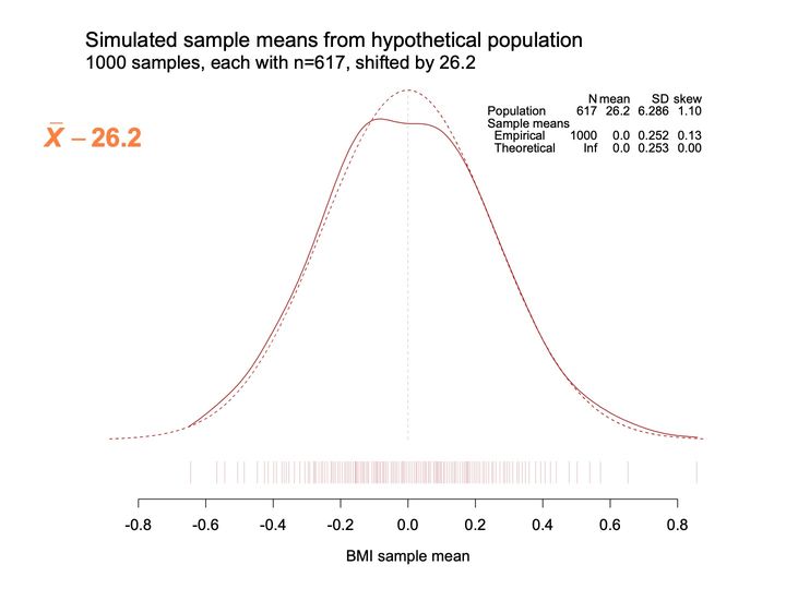
- The same 2 curves as before, now centered on the reference line at 0.0: a smooth symmetric dashed bell and a solid curve that is lower and flatter on top, slightly outside the bell on the left flank and slightly above it in the right tail. The ticks are densest between about -0.4 and 0.3, with the right end trailing further than the left.
Text in the picture
Simulated sample means from hypothetical population
1000 samples, each with n=617, shifted by 26.2
x̄ − 26.2
N mean SD skew
Population 617 26.2 6.286 1.10
Sample means
Empirical 1000 0.0 0.252 0.13
Theoretical Inf 0.0 0.253 0.00
Abbreviations: BMI = body mass index (kg/m²); SD = standard deviation.
- Panels
- 1
- Elements
- 2 dark red density curves (1 solid, 1 dashed) above a rug of thin pink vertical ticks depict sample means; a faint gray dashed vertical reference line
- Horizontal
- Labeled BMI sample mean, -3.5 to 3.5 in steps of 0.5; reference line at 0.0; ticks run from about -2.55 to about 3.4; the dashed curve spans the full axis
- Vertical
- No vertical axis or scale; the dashed curve's peak reaches the top of the plotting area
- Visible pattern
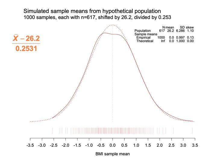
- The 2 curves keep their shapes, centered on 0.0, with the dashed bell symmetric and the solid curve lower and flatter on top and slightly heavier in the right tail. The dashed curve approaches zero height near both ends of the axis. The ticks are densest between about -1.5 and 1.2, with a longer trail to the right.
Text in the picture
Simulated sample means from hypothetical population
1000 samples, each with n=617, shifted by 26.2, divided by 0.253
(x̄ − 26.2) / 0.2531
N mean SD skew
Population 617 26.2 6.286 1.10
Sample means
Empirical 1000 0.0 0.997 0.13
Theoretical Inf 0.0 1.000 0.00
Abbreviations: BMI = body mass index (kg/m²); SD = standard deviation.
- Panels
- 1
- Elements
- 2 dark red density curves (1 solid, 1 dashed) above a rug of thin pink vertical ticks; a gray-filled area under the dashed density curve; 2 faint gray dashed vertical reference lines; an orange label with an orange arrow pointing into the gray area
- Horizontal
- Labeled BMI sample mean, -3.5 to 3.5 in steps of 0.5; reference lines at 0.0 and at about -1.645; the gray area spans from the left end of the axis to the line at about -1.645
- Vertical
- No vertical axis or scale; the dashed curve's peak reaches the top of the plotting area
- Visible pattern
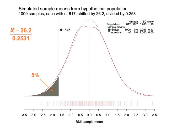
- The curves and ticks are as on the previous slide. The gray area fills the left tail under the dashed curve, rising from near zero height at -3.5 to about a quarter of the peak height at the cutoff near -1.645.
Text in the picture
Simulated sample means from hypothetical population
1000 samples, each with n=617, shifted by 26.2, divided by 0.253
(x̄ − 26.2) / 0.2531
−1.645
5%
N mean SD skew
Population 617 26.2 6.286 1.10
Sample means
Empirical 1000 0.0 0.997 0.13
Theoretical Inf 0.0 1.000 0.00
Abbreviations: BMI = body mass index (kg/m²); SD = standard deviation.
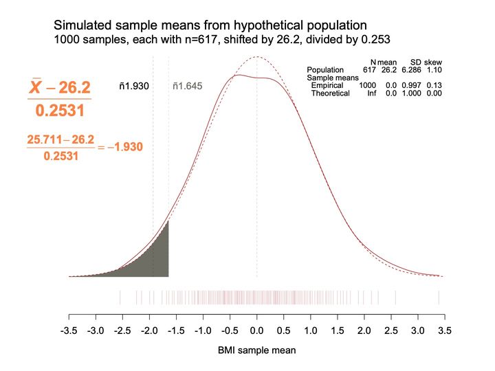
- Panels
- 1
- Elements
- 2 dark red density curves (1 solid, 1 dashed) above a rug of thin pink vertical ticks; a gray-filled area under the dashed density curve; 3 dashed vertical reference lines, 2 faint gray and one darker inside the gray area
- Horizontal
- Labeled BMI sample mean, -3.5 to 3.5 in steps of 0.5; reference lines at 0.0, about -1.645 and about -1.93; the gray area spans from the left end of the axis to about -1.645
- Vertical
- No vertical axis or scale; the dashed curve's peak reaches the top of the plotting area
- Visible pattern
- The gray left tail ends at the cutoff near -1.645, as before. A second line, at about -1.93, lies a short distance further left and passes through the gray area, where the curve is a little lower. The label for -1.930 is black and the label for -1.645 is gray.
Text in the picture
Simulated sample means from hypothetical population
1000 samples, each with n=617, shifted by 26.2, divided by 0.253
(x̄ − 26.2) / 0.2531
(25.711 − 26.2) / 0.2531 = −1.930
−1.930
−1.645
N mean SD skew
Population 617 26.2 6.286 1.10
Sample means
Empirical 1000 0.0 0.997 0.13
Theoretical Inf 0.0 1.000 0.00
Abbreviations: BMI = body mass index (kg/m²); SD = standard deviation.
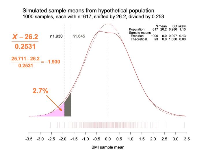
- Panels
- 1
- Elements
- 2 dark red density curves (1 solid, 1 dashed) above a rug of thin pink vertical ticks; under the dashed density curve a pink-filled area and a gray-filled area; 3 faint dashed vertical reference lines; an orange label with an orange arrow pointing into the pink area
- Horizontal
- Labeled BMI sample mean, -3.5 to 3.5 in steps of 0.5; reference lines at 0.0, about -1.645 and about -1.93; pink area from the left end of the axis to about -1.93, gray area from about -1.93 to about -1.645
- Vertical
- No vertical axis or scale; the dashed curve's peak reaches the top of the plotting area
- Visible pattern
- The left tail under the dashed curve is now divided at the line near -1.93: the larger, lower part to its left is pink, and a narrow gray strip remains between -1.93 and -1.645. The rest of the plot is unchanged from the previous slide.
Text in the picture
Simulated sample means from hypothetical population
1000 samples, each with n=617, shifted by 26.2, divided by 0.253
(x̄ − 26.2) / 0.2531
(25.711 − 26.2) / 0.2531 = −1.930
−1.930
−1.645
2.7%
N mean SD skew
Population 617 26.2 6.286 1.10
Sample means
Empirical 1000 0.0 0.997 0.13
Theoretical Inf 0.0 1.000 0.00
Abbreviations: BMI = body mass index (kg/m²); SD = standard deviation.
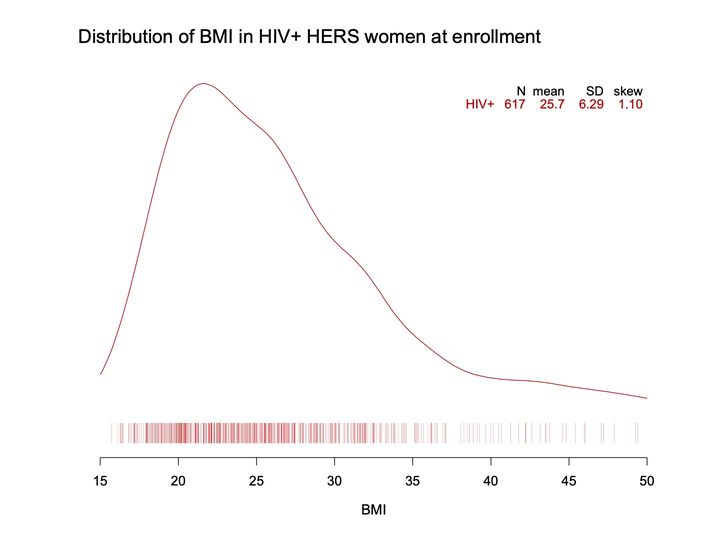
- Panels
- 1
- Elements
- 1 solid red density curve above a rug of thin red vertical ticks; both depict BMI values
- Horizontal
- BMI, 15 to 50 in steps of 5; the curve spans the full axis; ticks run from about 16 to about 49.5
- Vertical
- No vertical axis or scale; the curve's peak reaches near the top of the plotting area
- Visible pattern
- The curve rises steeply from the left end of the axis to a single peak near 21.5, then falls more slowly, with slight shoulders near 26 and 31. Beyond about 38 it flattens into a long, low right tail that declines gently to 50. The ticks are dense from about 16 to 33, thinner to about 37, and widely scattered from about 38 to 49.5.
Text in the picture
Distribution of BMI in HIV+ HERS women at enrollment
N mean SD skew
HIV+ 617 25.7 6.29 1.10
Abbreviations: BMI = body mass index (kg/m²); HER/HERS = HIV Epidemiology Research (HER) Study; HIV+ = HIV-positive; SD = standard deviation.
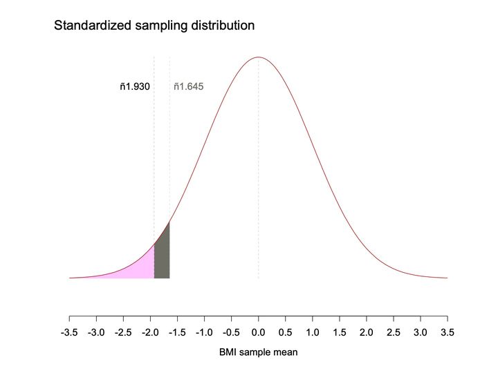
- Panels
- 1
- Elements
- 1 solid dark red bell curve; under it a pink-filled area and a gray-filled area; 3 faint dashed vertical reference lines; no rug and no table
- Horizontal
- Labeled BMI sample mean, -3.5 to 3.5 in steps of 0.5; reference lines at 0.0, about -1.645 and about -1.93; pink area from the left end of the axis to about -1.93, gray area from about -1.93 to about -1.645
- Vertical
- No vertical axis or scale; the curve's peak reaches the top of the plotting area
- Visible pattern
- The curve is a single symmetric bell centered on the line at 0.0, approaching zero height at both ends of the axis. The left tail beyond about -1.93 is pink, and a narrow gray strip lies between -1.93 and -1.645, where the curve stands at about a quarter of its peak height.
Text in the picture
Standardized sampling distribution
−1.930
−1.645
Abbreviations: BMI = body mass index (kg/m²).
Abbreviations: BMI = body mass index (kg/m²); HIV = human immunodeficiency virus; HIV+ = HIV-positive; SD = standard deviation.
Abbreviations: BMI = body mass index (kg/m²); HIV = human immunodeficiency virus; HIV+ = HIV-positive; SD = standard deviation.
Abbreviations: BMI = body mass index (kg/m²); HIV = human immunodeficiency virus; HIV+ = HIV-positive; SD = standard deviation.
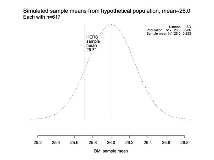
- Panels
- 1
- Elements
- 1 dashed dark red bell curve; 2 faint gray dashed vertical reference lines, one with a stacked text label; no rug
- Horizontal
- BMI sample mean, 25.2 to 26.8 in steps of 0.2; reference lines at 26.0 and at about 25.71; the curve extends slightly past both ends of the axis
- Vertical
- No vertical axis or scale; the curve's peak reaches the top of the plotting area
- Visible pattern
- The curve is a single symmetric bell centered on the line at 26.0, approaching zero height near both ends of the axis. The labeled line at about 25.71 crosses the left flank at roughly half the peak height.
Text in the picture
Simulated sample means from hypothetical population, mean=26.0
Each with n=617
HERS
sample
mean
25.71
N mean SD
Population 617 26.0 6.286
Sample mean Inf 26.0 0.253
Abbreviations: BMI = body mass index (kg/m²); HER/HERS = HIV Epidemiology Research (HER) Study; SD = standard deviation.
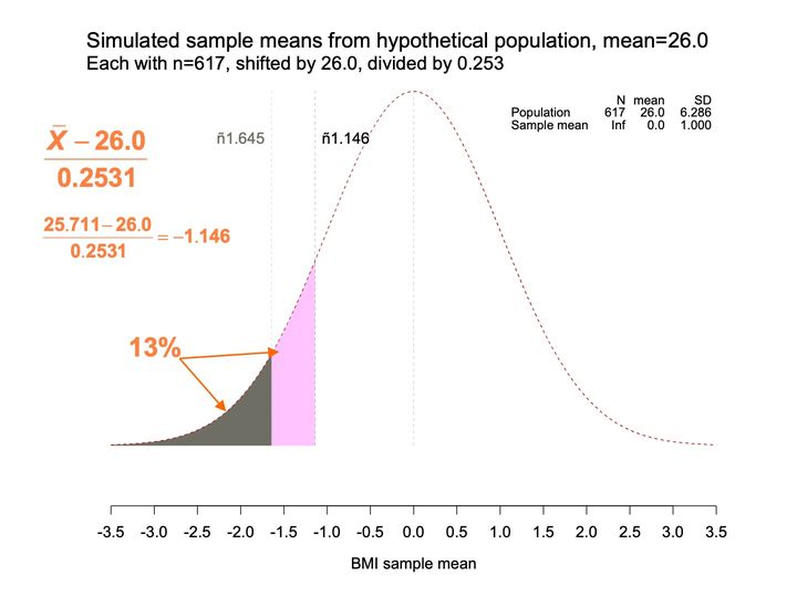
- Panels
- 1
- Elements
- 1 dashed dark red bell curve; under it a gray-filled area and a pink-filled area; 3 faint dashed vertical reference lines; an orange label with 2 orange arrows, one pointing into the gray area and one to the top of the boundary between the gray and pink areas
- Horizontal
- Labeled BMI sample mean, -3.5 to 3.5 in steps of 0.5; reference lines at 0.0, about -1.645 and about -1.146; gray area from the left end of the axis to about -1.645, pink area from about -1.645 to about -1.146
- Vertical
- No vertical axis or scale; the curve's peak reaches the top of the plotting area
- Visible pattern
- The curve is a single symmetric bell centered on the line at 0.0. The gray left tail ends at about -1.645, and a pink band continues to the right of it up to the line at about -1.146, where the curve stands at roughly half its peak height. Here the line at -1.146 lies to the right of the line at -1.645, and its label is black while the -1.645 label is gray.
Text in the picture
Simulated sample means from hypothetical population, mean=26.0
Each with n=617, shifted by 26.0, divided by 0.253
(x̄ − 26.0) / 0.2531
(25.711 − 26.0) / 0.2531 = −1.146
−1.645
−1.146
13%
N mean SD
Population 617 26.0 6.286
Sample mean Inf 0.0 1.000
Abbreviations: BMI = body mass index (kg/m²); SD = standard deviation.
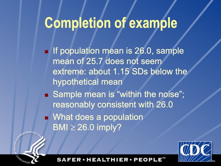
Abbreviations: BMI = body mass index (kg/m²); SD = standard deviation.
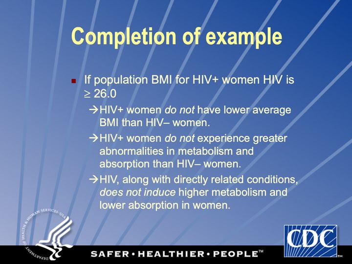
Abbreviations: BMI = body mass index (kg/m²); HIV = human immunodeficiency virus; HIV+ = HIV-positive.
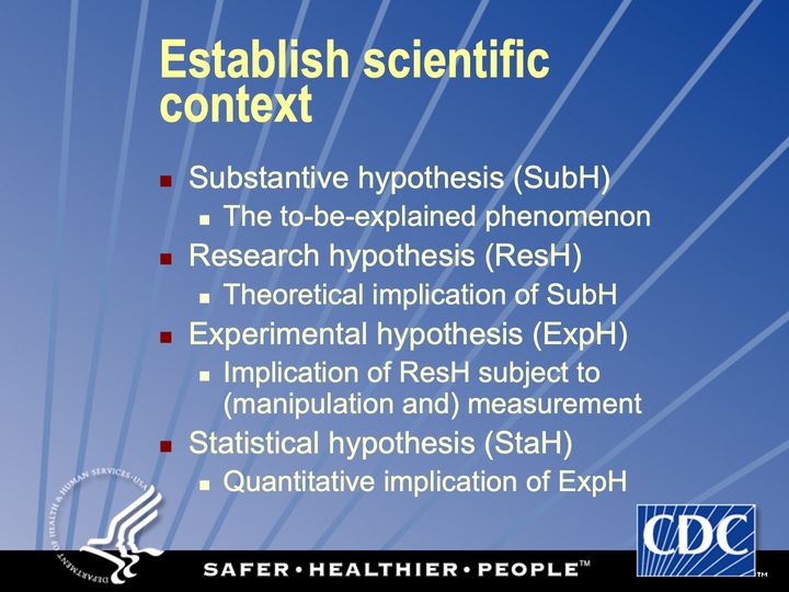
Abbreviations: ResH = research hypothesis; StaH = statistical hypothesis; SubH = substantive hypothesis.
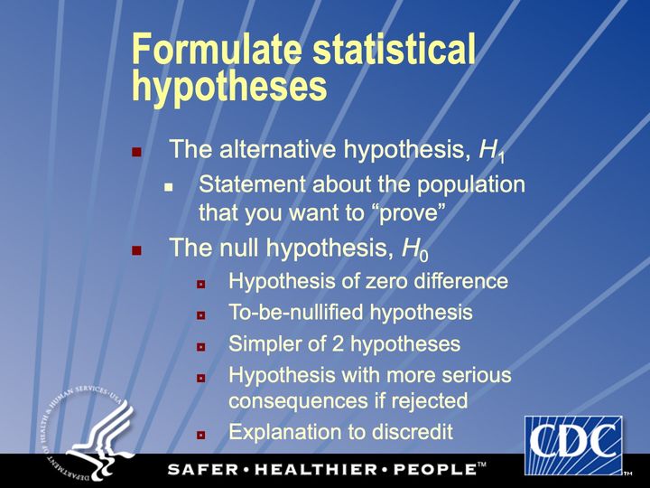
Simple: subtract and divide
Complex: intensive simulations
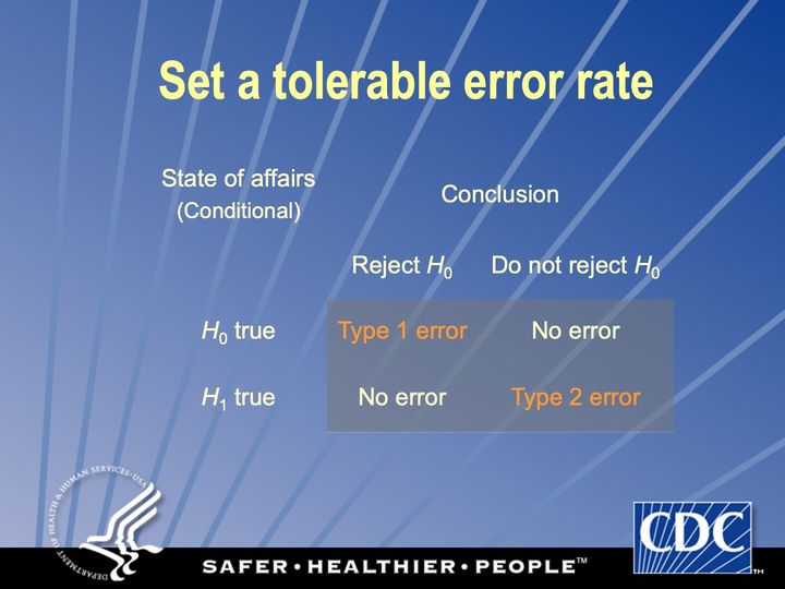
Conditional probability
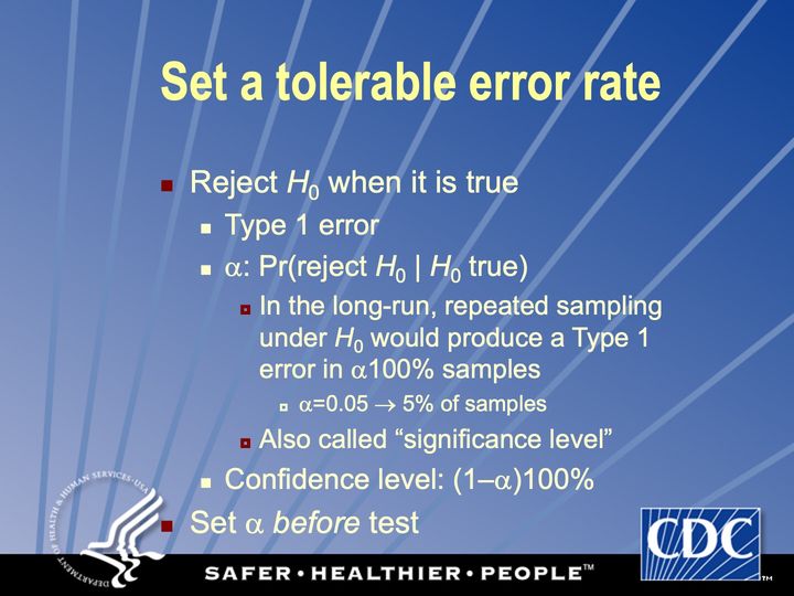
Conditional probability
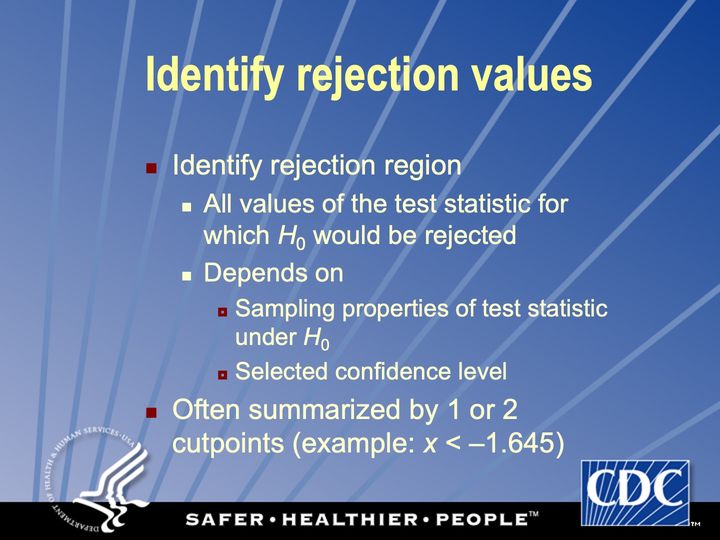
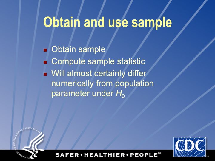
Conditional probability
Conditional probability
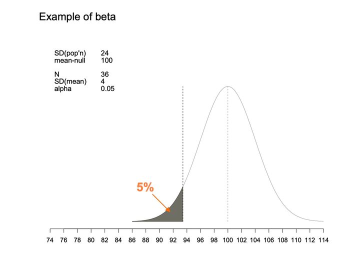
- Panels
- 1
- Elements
- 1 bell-shaped curve; a dashed vertical line at the curve's center and a second dashed vertical line at a cutpoint to its left; the area under the curve left of the cutpoint is shaded dark gray, with an orange arrow pointing into it from the label "5%"
- Horizontal
- 74 to 114 in steps of 2, unlabeled scale; the curve runs from about 86 to 114; dashed vertical guides at 100 and at about 93
- Vertical
- no axis, scale or labels
- Visible pattern
- A single symmetric curve rises from near zero at about 86 to its peak at 100 and falls back to near zero by 114. The thin left tail, from about 86 to the cutpoint at about 93, is shaded.
Text in the picture
Example of beta
SD(pop'n) 24
mean-null 100
N 36
SD(mean) 4
alpha 0.05
Abbreviations: SD = standard deviation.
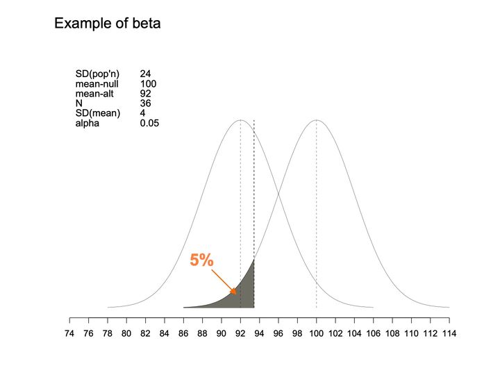
- Panels
- 1
- Elements
- 2 bell-shaped curves of the same width and height, each with a dashed vertical line at its center; a third dashed vertical line at a cutpoint; the area under the right-hand curve left of the cutpoint is shaded dark gray, with an orange arrow pointing into it from the label "5%"
- Horizontal
- 74 to 114 in steps of 2, unlabeled scale; the curves together run from about 78 to 114; dashed vertical guides at 92, at about 93 and at 100
- Vertical
- no axis, scale or labels; both peaks at the same height
- Visible pattern
- The left curve spans about 78 to 106 and peaks at 92; the right curve spans about 86 to 114 and peaks at 100. The 2 curves overlap broadly between about 86 and 106 and cross at about 96. The cutpoint lies just right of the left curve's peak, and the dark gray tail of the right curve, from about 86 to 93, sits inside the left curve's central region.
Text in the picture
Example of beta
SD(pop'n) 24
mean-null 100
mean-alt 92
N 36
SD(mean) 4
alpha 0.05
Abbreviations: SD = standard deviation.
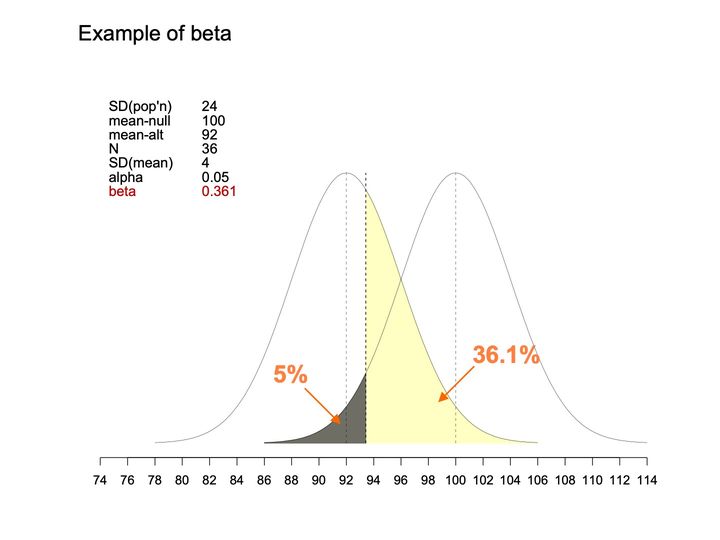
- Panels
- 1
- Elements
- 2 bell-shaped curves of the same width and height, each with a dashed vertical line at its center; a third dashed vertical line at a cutpoint; under the right-hand curve, the area left of the cutpoint is shaded dark gray, with an orange arrow from the label "5%"; under the left-hand curve, the area right of the cutpoint is shaded pale yellow, with an orange arrow from the label "36.1%"; a parameter table is placed at the upper left.
- Horizontal
- 74 to 114, ticks every 2; curves span about 78 to 114; thin dashed verticals at 92 and 100, bolder dashed vertical at about 93
- Vertical
- No axis or scale; both curves rise from a common baseline to the same peak height, with the parameter table to the left of the left curve's peak
- Visible pattern
- The curves are placed as on the previous slide: the left one spans about 78 to 106 and peaks at 92, the right one spans about 86 to 114 and peaks at 100, and they cross at about 96. The cutpoint at about 93 divides 2 shaded regions that meet along it: the small dark gray tail of the right curve to its left, from about 86, and the much larger yellow region of the left curve to its right, extending to about 106. The yellow region covers the left curve's whole right side beyond the cutpoint, including the area where the 2 curves overlap.
Text in the picture
Example of beta
SD(pop'n) 24
mean-null 100
mean-alt 92
N 36
SD(mean) 4
alpha 0.05
beta 0.361
Abbreviations: SD = standard deviation.

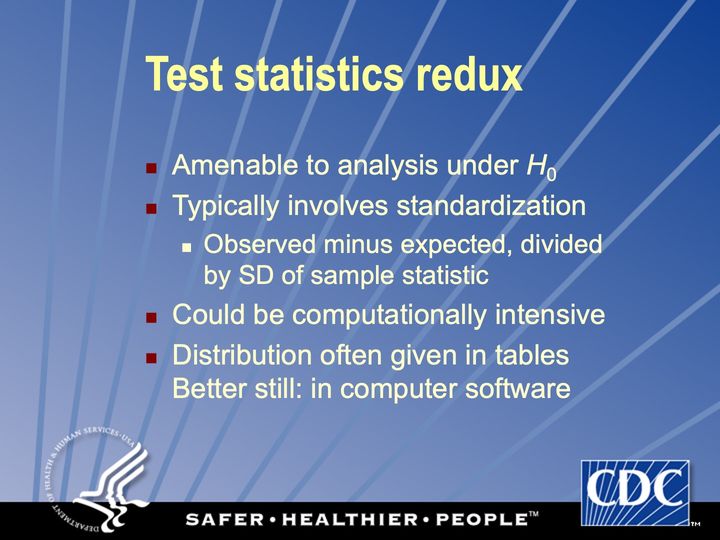
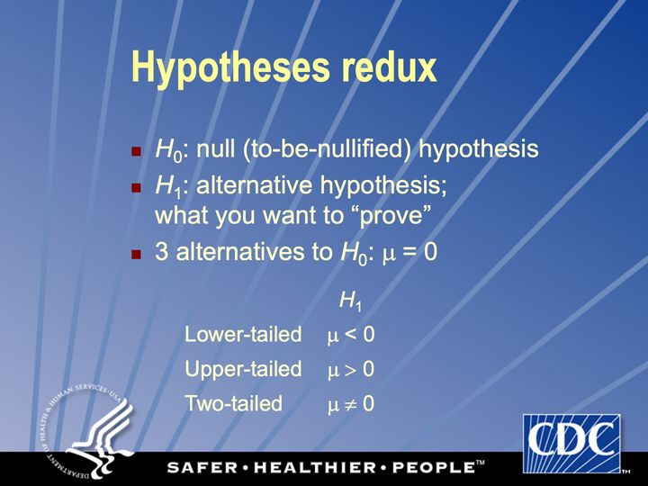
Observed minus expected (under H0), rescaled to unit variance (under H0)
Abbreviations: SD = standard deviation.
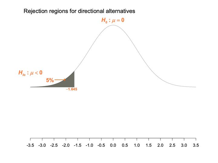
- Panels
- 1
- Elements
- 1 bell-shaped curve (thin black line); the area under its left tail is shaded dark gray, and an orange arrow labeled 5% points to the shaded area; orange labels give the hypotheses and the cutoff
- Horizontal
- -3.5 to 3.5, ticks every 0.5; the shaded area ends at -1.645, labeled beneath its right edge
- Vertical
- no axis or scale; the curve occupies the upper half of the plot area, and the lower half, above the horizontal axis, is empty
- Visible pattern
- The curve is symmetric, peaking above 0 and falling to a nearly flat baseline by -3.5 and 3.5. The shaded region is a thin wedge in the left tail, from -3.5 to about -1.6, rising toward its right edge where it meets the curve. Only the left side carries shading; the right tail is unshaded.
Text in the picture
Rejection regions for directional alternatives
H_0: μ = 0
H_lo: μ < 0
5%
−1.645
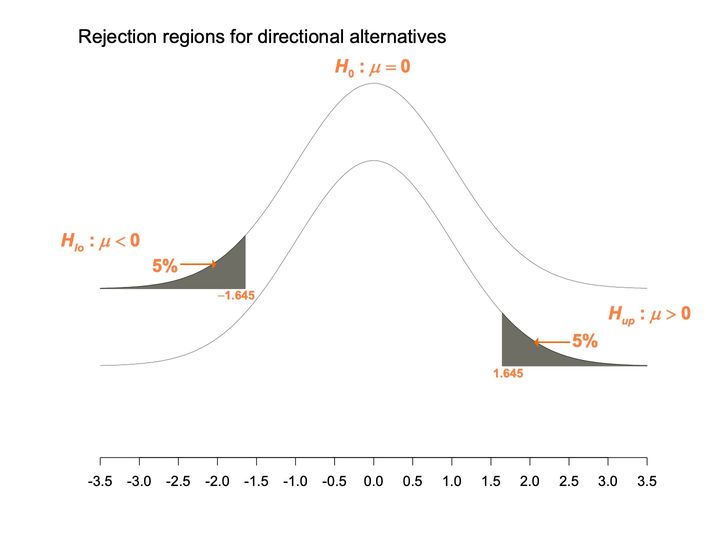
- Panels
- 1
- Elements
- 2 identical bell-shaped curves (thin black lines) offset vertically; dark gray shading under the left tail of the upper curve and under the right tail of the lower curve; orange arrows labeled 5% point to each shaded area; orange labels give the hypotheses and cutoffs
- Horizontal
- -3.5 to 3.5, ticks every 0.5; the upper curve's shading ends at -1.645 and the lower curve's begins at 1.645, each labeled
- Vertical
- no axis or scale; the 2 curves fill roughly the upper 3 quarters of the plot area, leaving empty space above the horizontal axis
- Visible pattern
- Both curves are symmetric and centered on 0, with the lower curve a copy of the upper one shifted down. The shaded regions mirror each other: a wedge from -3.5 to about -1.6 on the upper curve, and a wedge from about 1.6 to 3.5 on the lower curve. The hypothesis labels sit beside the tail they belong to, one at the left and one at the right.
Text in the picture
Rejection regions for directional alternatives
H_0: μ = 0
H_lo: μ < 0
5%
−1.645
H_up: μ > 0
5%
1.645
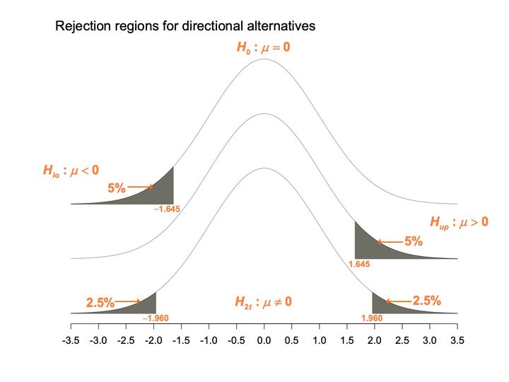
- Panels
- 1
- Elements
- 3 identical bell-shaped curves (thin black lines) offset vertically; dark gray shading under the left tail of the top curve, the right tail of the middle curve, and both tails of the bottom curve; orange arrows with percentage labels point to each shaded area; orange labels give the hypotheses and cutoffs
- Horizontal
- -3.5 to 3.5, ticks every 0.5; cutoffs labeled at -1.645 (top curve), 1.645 (middle curve), and -1.960 and 1.960 (bottom curve)
- Vertical
- no axis or scale; the bottom curve's baseline sits just above the horizontal axis
- Visible pattern
- All 3 curves are symmetric and centered on 0, each a copy of the one above shifted down by the same amounty. The top and middle curves each carry one wedge of shading, 5% each, in the left and right tails respectively, reaching in to about ±1.6. The bottom curve carries 2 smaller wedges, 2.5% each, beyond about ±2.0, with its hypothesis label placed beneath the center of the curve.
Text in the picture
Rejection regions for directional alternatives
H_0: μ = 0
H_lo: μ < 0
5%
−1.645
H_up: μ > 0
5%
1.645
2.5%
−1.960
H_2t: μ ≠ 0
2.5%
1.960
Not too non-normal: not too skewed, tails not too heavy; compensated by larger samples
If too non-normal: transformations, “distribution-free” tests
Text in the picture
17 59
GUINNESS
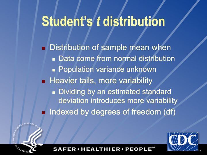
Degrees of freedom: # obs minus # independently estimated parameters
Invented by W S Gossett in 1908 at Guinness brewery, published under pseudonym at behest of brewery
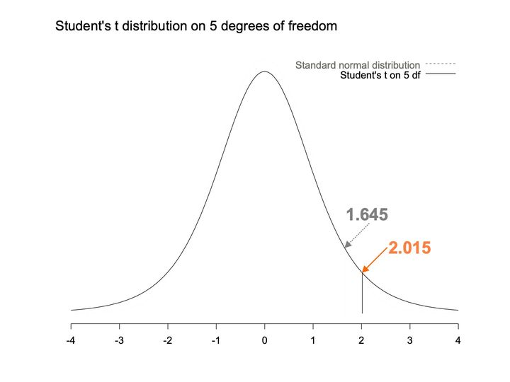
- Panels
- 1
- Elements
- 2 density curves: a dashed light gray curve (standard normal distribution) and a solid black curve (Student's t on 5 df), identified by a legend at upper right; a solid vertical line from the baseline up to the t curve; a dotted gray arrow labeled 1.645 and a solid orange arrow labeled 2.015 point to the right flank of the t curve
- Horizontal
- -4 to 4, integer ticks; the solid vertical line stands at about 2.0
- Vertical
- no axis or scale
- Visible pattern
- The solid t curve is bell-shaped and symmetric about 0, falling to a low, still slightly raised baseline at -4 and 4. The dashed normal curve is very faint; it can be seen just outside the solid curve near the peak, so its peak is a little higher, and is otherwise hard to tell apart. The 2 arrows point to neighboring spots on the right flank, the gray one at about 1.6 and the orange one at about 2.0, where the vertical line meets the curve.
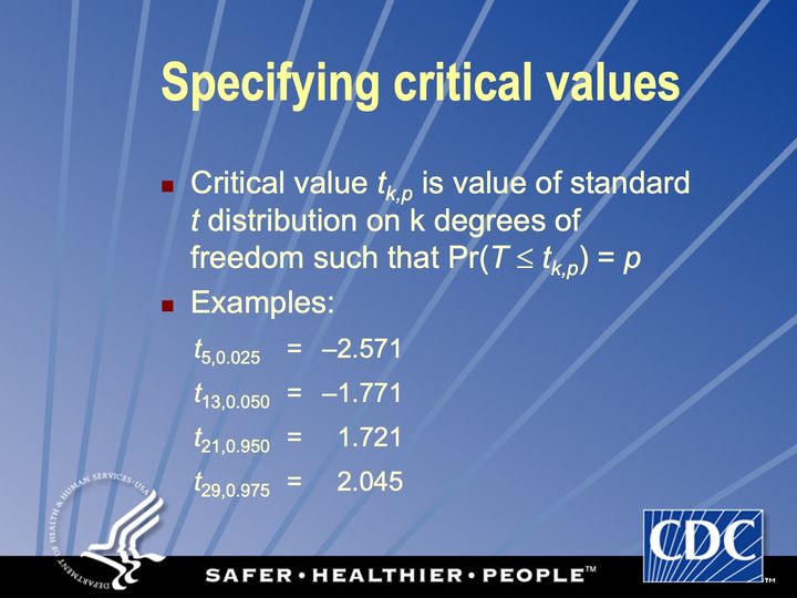
Text in the picture
Student's t distribution on 5 degrees of freedom
1.645
2.015
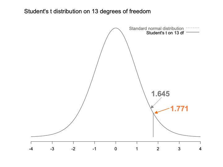
- Panels
- 1
- Elements
- 2 density curves named in a legend at upper right: standard normal distribution (dashed light gray) and Student's t on 13 df (solid black); a solid vertical line from the baseline up to the curve; a dotted gray arrow labeled 1.645 and a solid orange arrow labeled 1.771 point to the right flank of the curve
- Horizontal
- -4 to 4, integer ticks; the solid vertical line stands at about 1.8
- Vertical
- no axis or scale
- Visible pattern
- A single bell-shaped curve is visible, symmetric about 0 and falling to a nearly flat baseline by -4 and 4; the dashed normal curve cannot be told apart from it. The 2 arrows point to nearly the same place on the right flank, the gray one at about 1.6 and the orange one at about 1.8, where the vertical line meets the curve.
Text in the picture
Student's t distribution on 13 degrees of freedom
1.645
1.771
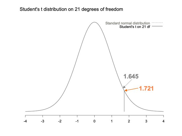
- Panels
- 1
- Elements
- 2 density curves named in a legend at upper right: standard normal distribution (dashed light gray) and Student's t on 21 df (solid black); a solid vertical line from the baseline up to the curve; a dotted gray arrow labeled 1.645 and a solid orange arrow labeled 1.721 point to the right flank of the curve
- Horizontal
- -4 to 4, integer ticks; the solid vertical line stands at about 1.7
- Vertical
- no axis or scale
- Visible pattern
- A single bell-shaped curve is visible, symmetric about 0 and falling to a nearly flat baseline by -4 and 4; the dashed normal curve cannot be told apart from it. The 2 arrows point to almost the same place on the right flank, at about 1.6 and 1.7, the orange one meeting the curve where the vertical line stands.
Text in the picture
Student's t distribution on 21 degrees of freedom
1.645
1.721
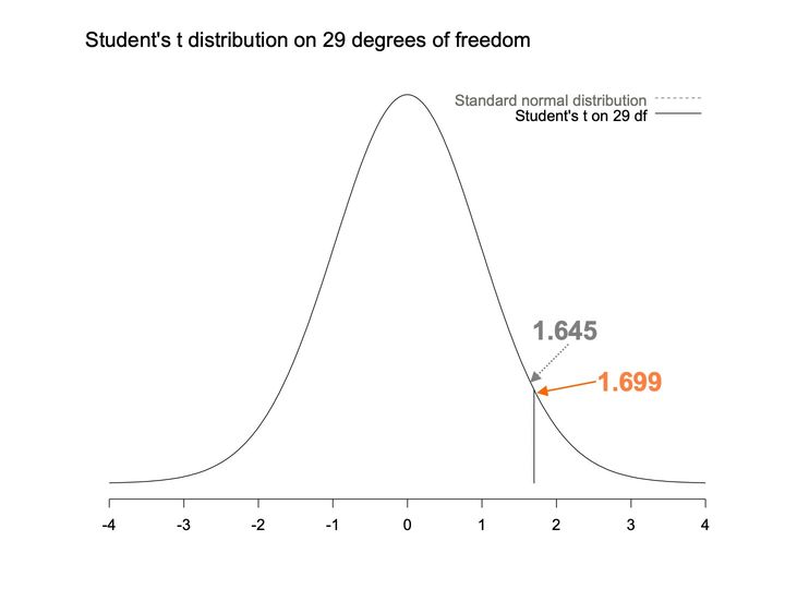
- Panels
- 1
- Elements
- 2 density curves named in a legend at upper right: standard normal distribution (dashed light gray) and Student's t on 29 df (solid black); a solid vertical line from the baseline up to the curve; a dotted gray arrow labeled 1.645 and a solid orange arrow labeled 1.699 point to the right flank of the curve
- Horizontal
- -4 to 4, integer ticks; the solid vertical line stands at about 1.7
- Vertical
- no axis or scale
- Visible pattern
- A single bell-shaped curve is visible, symmetric about 0 and falling to a nearly flat baseline by -4 and 4; the dashed normal curve cannot be told apart from it. The 2 arrows point to almost the same place on the right flank, at about 1.6 and 1.7, the orange one meeting the curve where the vertical line stands.
Text in the picture
Student's t distribution on 29 degrees of freedom
1.645
1.699
Text in the picture
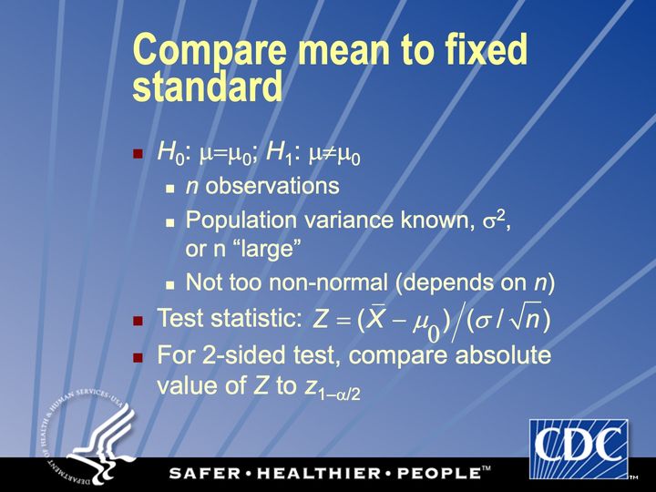
Z = (X-bar − μ_0) / (σ / sqrt(n))
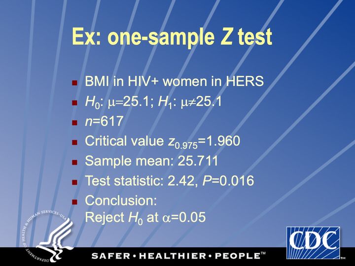
Abbreviations: BMI = body mass index (kg/m²); HER/HERS = HIV Epidemiology Research (HER) Study; HIV+ = HIV-positive.
Text in the picture
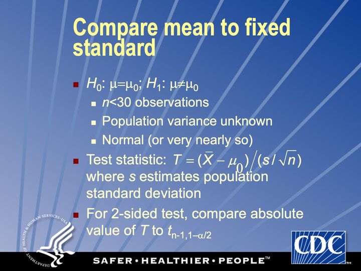
T = (X-bar − μ0) / (s / sqrt(n))
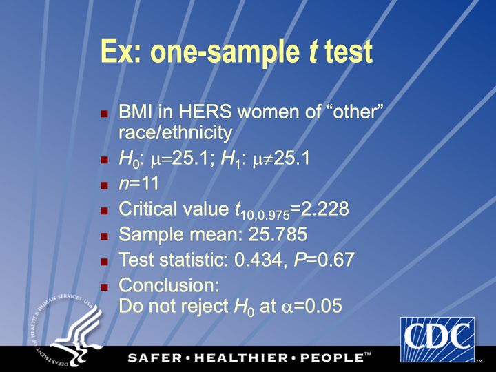
Abbreviations: BMI = body mass index (kg/m²); HER/HERS = HIV Epidemiology Research (HER) Study.
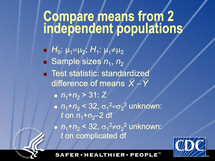
Text in the picture
X-bar − Y-bar
Use t test if n1+n2<32; the degrees of freedom for the t test are more complicated if population variances are unequal
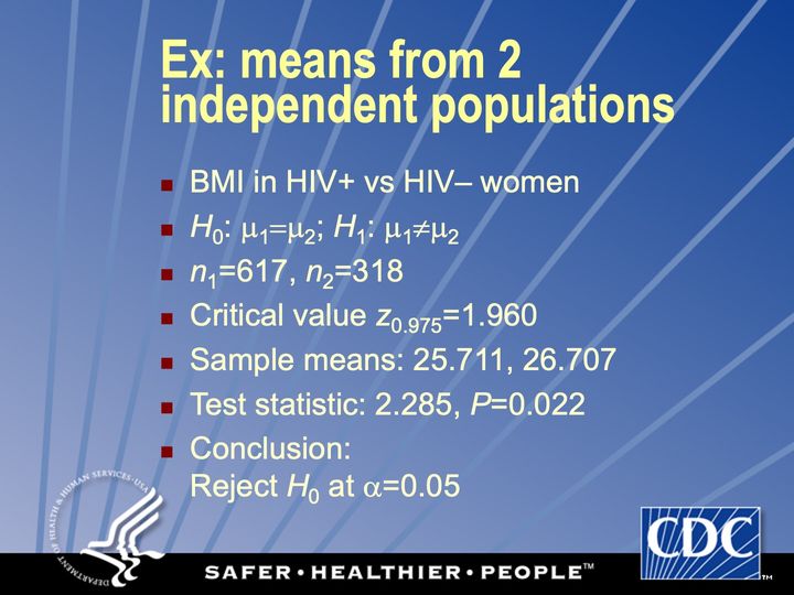
Abbreviations: BMI = body mass index (kg/m²); HIV = human immunodeficiency virus; HIV+ = HIV-positive.
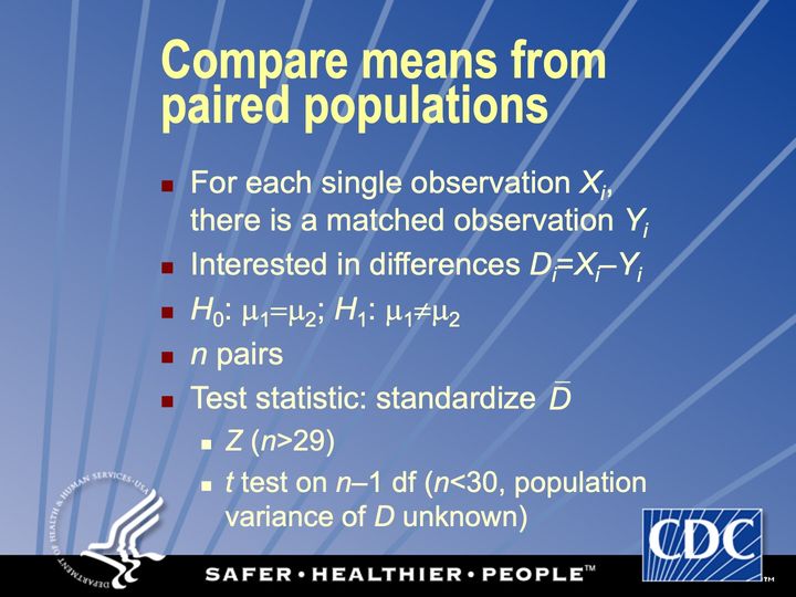
Text in the picture
D-bar
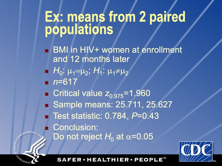
Abbreviations: BMI = body mass index (kg/m²); HIV+ = HIV-positive.
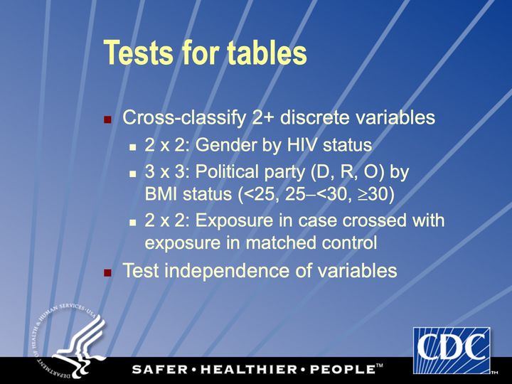
Abbreviations: BMI = body mass index (kg/m²); HIV = human immunodeficiency virus.
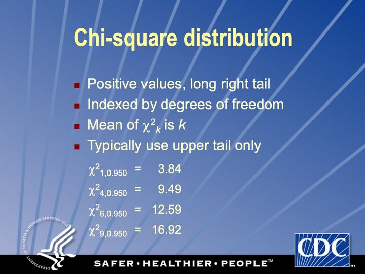
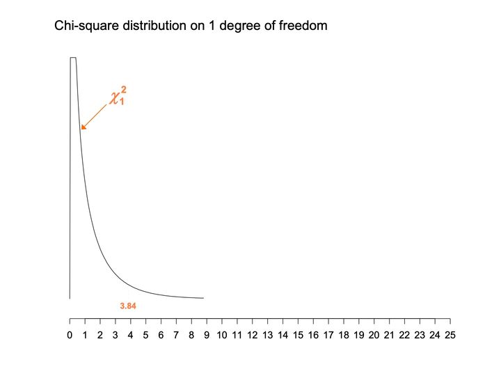
- Panels
- 1
- Elements
- 1 black curve, labeled chi-square with subscript 1 by an orange label and arrow; the value 3.84 in orange below the curve, with a faint short vertical line above it
- Horizontal
- 0 to 25, ticks and labels every 1; the curve spans 0 to about 9
- Vertical
- No axis, scale or labels; the curve is cut off flat at the top of the plotting area
- Visible pattern
- The curve rises almost vertically at 0 to the top of the plotting area, runs flat there for a short stretch to about 0.4, then falls steeply. By about 4 it lies close to the baseline, and it trails off nearly flat to its end near 9. The rest of the axis, to 25, is empty.
Text in the picture
Chi-square distribution on 1 degree of freedom
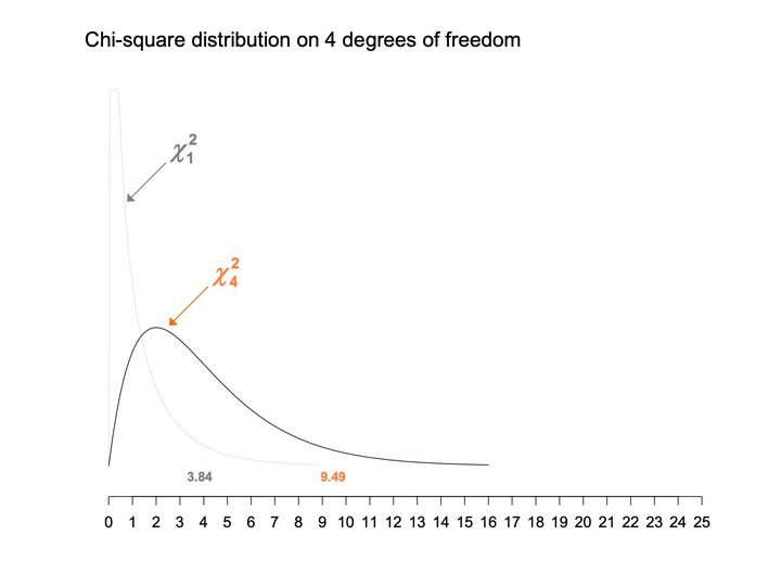
- Panels
- 1
- Elements
- 2 curves: chi-square with subscript 1 as a thin light gray line with a gray label and arrow, chi-square with subscript 4 as a black line with an orange label and arrow; the values 3.84 (gray) and 9.49 (orange) below the curves, each with a faint short vertical line above it
- Horizontal
- 0 to 25, ticks and labels every 1; the curves span 0 to about 16
- Vertical
- No axis, scale or labels; the gray curve is cut off flat at the top of the plotting area
- Visible pattern
- The gray curve keeps the shape of the previous chart: a near-vertical spike at 0, cut off at the top, falling steeply to the baseline. The black curve starts at 0, rises to a single rounded peak near 2 at about a third of the plotting height, and falls away in a long right tail that reaches the baseline near 16. The 2 curves cross near 1.3.
Text in the picture
Chi-square distribution on 4 degrees of freedom
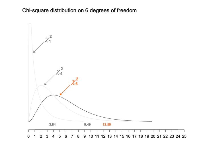
- Panels
- 1
- Elements
- 3 curves: chi-square with subscripts 1 and 4 as thin light gray lines with gray labels and arrows, chi-square with subscript 6 as a black line with an orange label and arrow; the values 3.84 and 9.49 (gray) and 12.59 (orange) below the curves, each with a faint short vertical line above it
- Horizontal
- 0 to 25, ticks and labels every 1; the curves span 0 to about 20
- Vertical
- No axis, scale or labels; the 1 curve is cut off flat at the top of the plotting area
- Visible pattern
- The 2 gray curves repeat the earlier charts. The black curve leaves 0 flat, rises to a rounded peak near 4 at about a quarter of the plotting height, lower than the gray 4 curve's peak, and declines in a long right tail to the baseline near 20. Each successive curve peaks further right, lower and wider.
Text in the picture
Chi-square distribution on 6 degrees of freedom
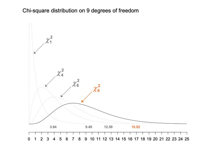
- Panels
- 1
- Elements
- 4 curves: chi-square with subscripts 1, 4 and 6 as thin light gray lines with gray labels and arrows, chi-square with subscript 9 as a black line with an orange label and arrow; the values 3.84, 9.49 and 12.59 (gray) and 16.92 (orange) below the curves, each with a faint short vertical line above it
- Horizontal
- 0 to 25, ticks and labels every 1; the black curve runs to the right end of the axis
- Vertical
- No axis, scale or labels; the 1 curve is cut off flat at the top of the plotting area
- Visible pattern
- The 3 gray curves repeat the earlier charts. The black curve stays near the baseline at first, rises to a broad rounded peak near 7 at about a fifth of the plotting height, the lowest of the 4 peaks, and declines slowly to near the baseline at 25. Across the 4 curves the peaks step rightward and downward, and the curves spread wider; the marked values step rightward with them.
Text in the picture
Chi-square distribution on 9 degrees of freedom
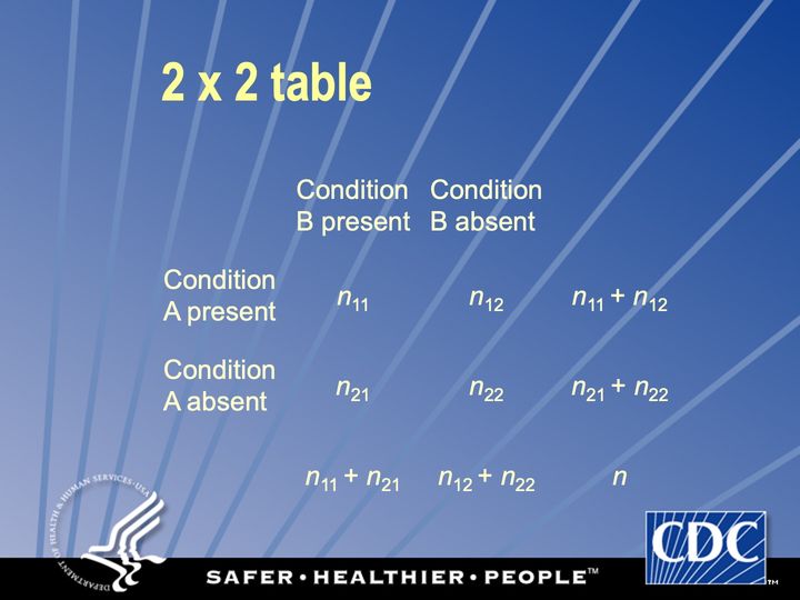
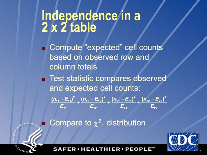
Text in the picture
(n11 − E11)^2 / E11 + (n12 − E12)^2 / E12 + (n21 − E21)^2 / E21 + (n22 − E22)^2 / E22
Odds ratio, prevalence ratio
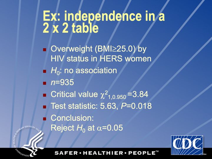
Abbreviations: BMI = body mass index (kg/m²); HER/HERS = HIV Epidemiology Research (HER) Study; HIV = human immunodeficiency virus.
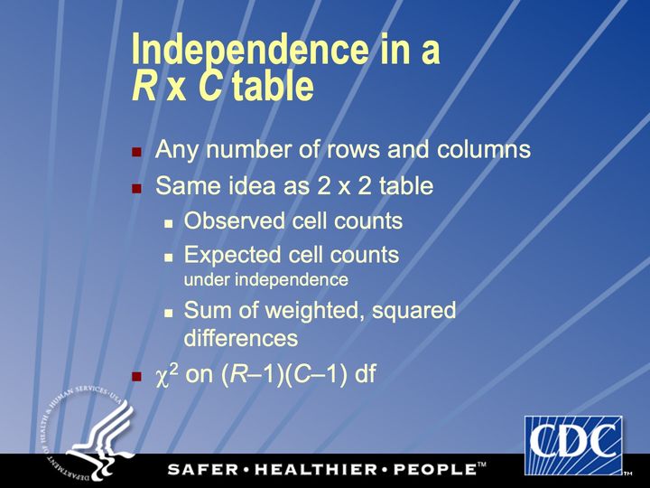
Correction available if expected counts of some cells are too small
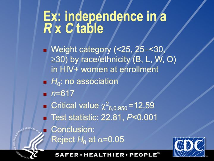
Abbreviations: HIV+ = HIV-positive.
Often highly discrete
Often highly discrete
Abbreviations: HIV+ = HIV-positive.
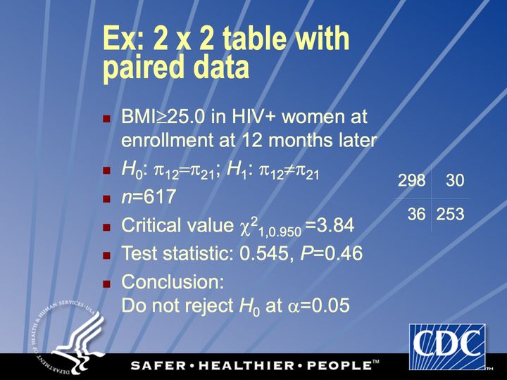
Continuity correction: TS: 0.379, P=0.54
Exact: P=0.54
Abbreviations: BMI = body mass index (kg/m²); HIV+ = HIV-positive; TS = test statistic.
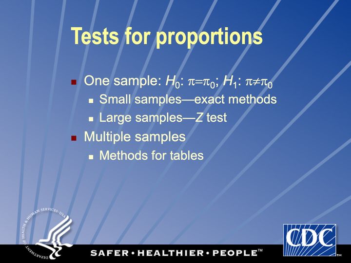
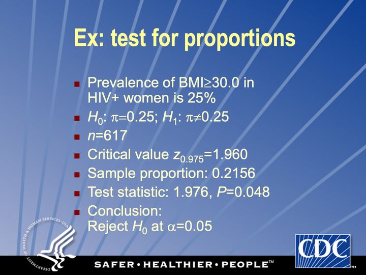
Abbreviations: BMI = body mass index (kg/m²); HIV+ = HIV-positive.
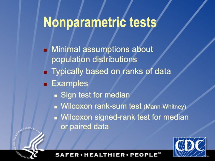
“distribution-free” “rank-based”
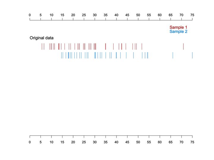
- Panels
- 1, unframed, with one labeled band of 2 rows
- Elements
- Vertical tick marks (a rug) depict individual values, red for Sample 1 (upper row) and blue for Sample 2 (lower row), with a 2-line color legend at upper right
- Horizontal
- 0 to 75, labeled every 5, axis repeated at top and bottom
- Vertical
- No scale; a single band labeled Original data near the top
- Visible pattern
- The red marks run from about 5 to about 52, most densely between about 5 and 31, with one isolated mark near 71. The blue marks begin later, at about 15, and run to about 55, with 2 isolated marks near 66 and 75. The 2 rows overlap across most of the middle range, but the red row extends further to the left and the blue row further to the right.
Text in the picture
Sample 1
Sample 2
Original data
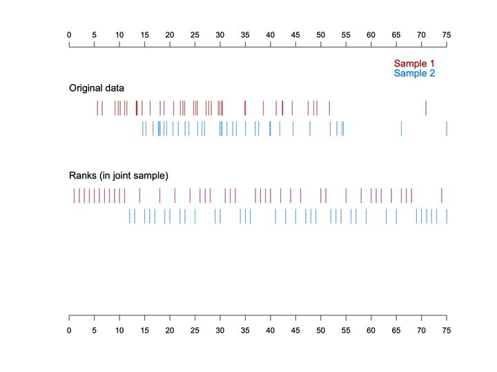
- Panels
- 1, unframed, with 2 labeled bands of 2 rows each
- Elements
- Vertical tick marks depict individual values (upper band) and their ranks (lower band), red for Sample 1 (upper row of each band) and blue for Sample 2 (lower row), with a 2-line color legend at upper right
- Horizontal
- 0 to 75, labeled every 5, axis repeated at top and bottom, serving as the value scale for the upper band and the rank scale for the lower band; ranks run from 1 to 75
- Vertical
- No scale; bands labeled Original data and Ranks (in joint sample), stacked top to bottom
- Visible pattern
- The upper band repeats the original values: red from about 5 to 52 with an outlier near 71, blue from about 15 to 55 with outliers near 66 and 75. In the rank band the marks fall on evenly spaced integer positions. Red holds an unbroken run of the lowest ranks, about 1 to 11, and blue begins at about 12; above that the colors interleave in short runs, with blue holding most of the highest ranks, about 69 to 75, apart from one red mark near 74. Overall the red ranks lean toward the left and the blue ranks toward the right.
Text in the picture
Sample 1
Sample 2
Original data
Ranks (in joint sample)
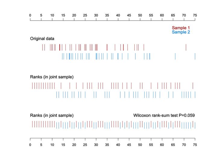
- Panels
- 1, unframed, with 3 labeled bands
- Elements
- Vertical tick marks depict individual values (top band) and ranks (middle and bottom bands), red for Sample 1 and blue for Sample 2; the top 2 bands keep the samples in separate rows, the bottom band merges them into a single row with blue marks set slightly lower than red; a 2-line color legend at upper right
- Horizontal
- 0 to 75, labeled every 5, axis repeated at top and bottom, serving as the value scale for the top band and the rank scale for the lower 2; ranks run from 1 to 75
- Vertical
- No scale; bands labeled Original data, Ranks (in joint sample), and Ranks (in joint sample) again, stacked top to bottom; the P-value annotation sits at the right above the bottom band
- Visible pattern
- The top 2 bands repeat the previous slide. In the bottom band all 75 ranks form one continuous evenly spaced row in which the colors alternate: a solid run of red from rank 1 to about 11, then a mix of short red and blue runs across the middle, and mostly blue at the far right, about 69 to 75, with one red mark near 74. Red marks are more frequent in the left half of the row and blue marks in the right half.
Text in the picture
Sample 1
Sample 2
Original data
Ranks (in joint sample)
Ranks (in joint sample)
Wilcoxon rank-sum test P=0.059

Jean Rostand (1894–1977), French biologist, writer. Pensées d’un Biologiste, ch. 10, “A Biologist’s Thoughts” (1939; repr. in The Substance of Man, 1962).
Marquis de Sade (1740–1814), French author. Mme Delbène, in L’Histoire de Juliette, ou les Prospérités du Vice, pt. 1 (1797).

Independent tests
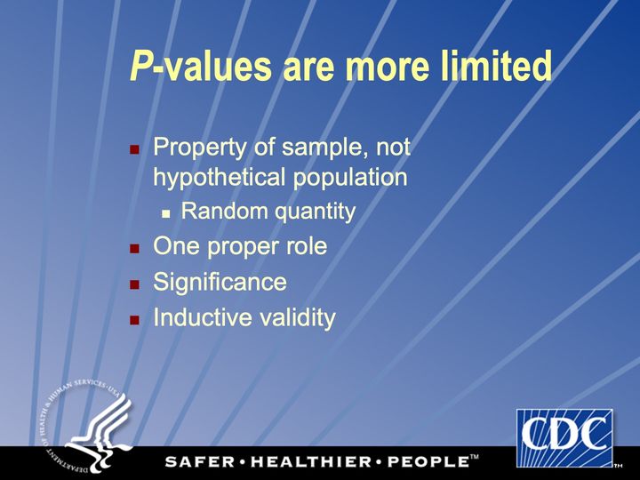
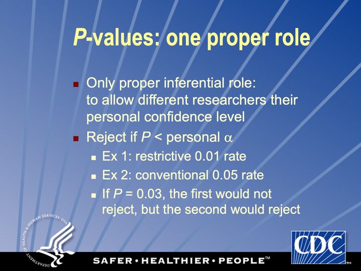
Have you hugged your inner α today?
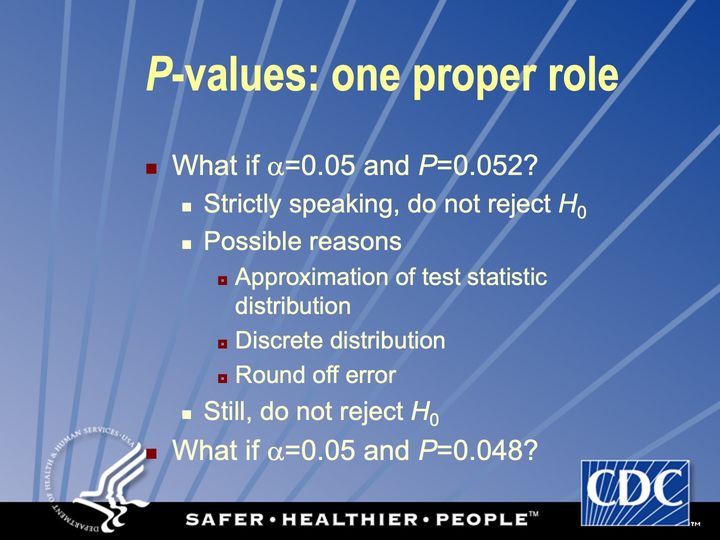
Have you hugged your inner α today?
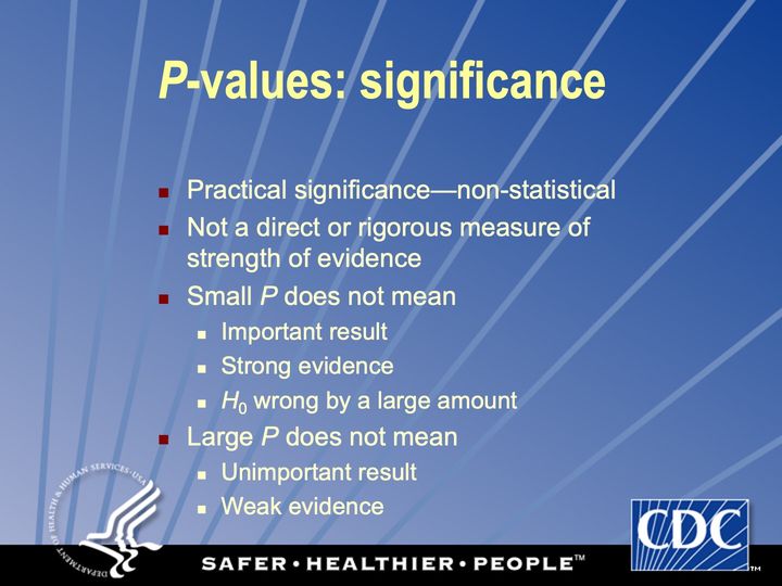
For a true measure of evidence, other statistical methods must be used
It’s all about chance
Define method of difference
Causality is a non-statistical concept: no test by itself can prove causality
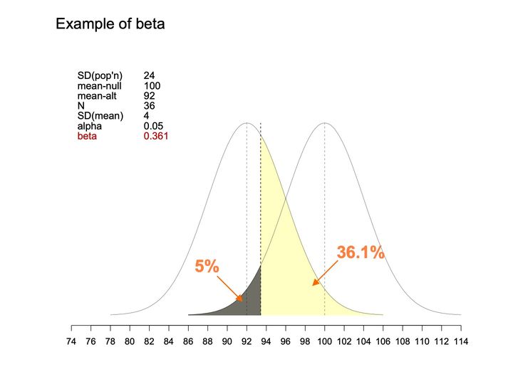
- Panels
- 1
- Elements
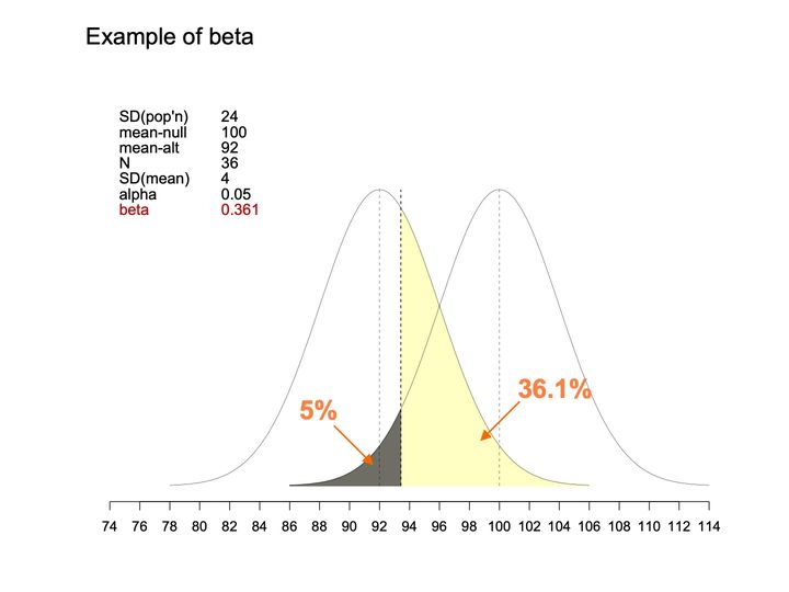
- 2 bell-shaped curves of the same width and height, each with a dashed vertical line at its center; a third dashed vertical line at a cutpoint; under the right-hand curve, the area left of the cutpoint is shaded dark gray, with an orange arrow from the label "5%"; under the left-hand curve, the area right of the cutpoint is shaded pale yellow, with an orange arrow from the label "36.1%"; a parameter table is placed at the upper left.
- Horizontal
- 74 to 114, ticks every 2; curves span about 78 to 114; thin dashed verticals at 92 and 100, bolder dashed vertical at about 93
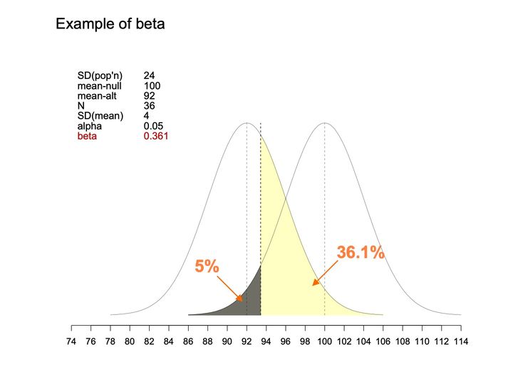
- Vertical
- No axis or scale; both curves rise from a common baseline to the same peak height, with the parameter table to the left of the left curve's peak
- Visible pattern
- The 2 curves overlap broadly, one peaked at 92 and the other at 100, crossing at about 96. The bolder dashed line at about 93 divides the shading: dark gray on the left , pale yellow on the right. An arrow labeled 5% points into the gray region, and an arrow labeled 36.1% points into the yellow region.
Text in the picture
Example of beta
SD(pop'n) 24
mean-null 100
mean-alt 92
N 36
SD(mean) 4
alpha 0.05
beta 0.361
Abbreviations: SD = standard deviation.
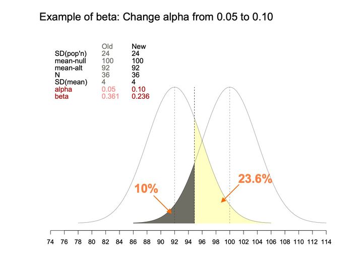
- Panels
- 1
- Elements
- 2 bell-shaped curve outlines of the same width and height; 2 shaded areas under them (dark gray, pale yellow); 3 dashed vertical lines (thin lines at each curve's peak, a bolder line between them); 2 orange arrows with percentage labels pointing into the shaded areas
- Horizontal
- Unlabeled number line, 74 to 114, ticks every 2; curves span about 78 to 114; thin dashed verticals at 92 and 100, bolder dashed vertical at about 95
- Vertical
- No axis or scale; both curves rise from a common baseline to the same peak height
- Visible pattern
- The same 2 overlapping curves, peaked at 92 and 100 and crossing at about 96, with the bolder dashed line now further right, at about 95. The dark gray region under the left tail of the curve peaked at 100 is larger than before, running from about 86 to 95; the pale yellow region under the curve peaked at 92 is smaller, running from about 95 to about 106. The arrow labeled 10% points into the gray region, and the arrow labeled 23.6% points into the yellow region. In the table, the Old column is in lighter gray, the alpha and beta rows are in red (Old values a paler red), and only those 2 rows differ between Old and New.
Text in the picture
Example of beta: Change alpha from 0.05 to 0.10
Old New
SD(pop'n) 24 24
mean-null 100 100
mean-alt 92 92
N 36 36
SD(mean) 4 4
alpha 0.05 0.10
beta 0.361 0.236
10%
23.6%
Abbreviations: SD = standard deviation.
- Panels
- 1
- Elements
- 2 bell-shaped curves of the same width and height, each with a dashed vertical line at its center; a third dashed vertical line at a cutpoint; under the right-hand curve, the area left of the cutpoint is shaded dark gray, with an orange arrow from the label "5%"; under the left-hand curve, the area right of the cutpoint is shaded pale yellow, with an orange arrow from the label "36.1%"; a parameter table is placed at the upper left.
- Horizontal
- 74 to 114, ticks every 2; curves span about 78 to 114; thin dashed verticals at 92 and 100, bolder dashed vertical at about 93
- Vertical
- No axis or scale; both curves rise from a common baseline to the same peak height, with the parameter table to the left of the left curve's peak
- Visible pattern
- The 2 curves overlap broadly, one peaked at 92 and the other at 100, crossing at about 96. The bolder dashed line at about 93 divides the shading: dark gray on the left , pale yellow on the right. An arrow labeled 5% points into the gray region, and an arrow labeled 36.1% points into the yellow region.
Text in the picture
Example of beta
SD(pop'n) 24
mean-null 100
mean-alt 92
N 36
SD(mean) 4
alpha 0.05
beta 0.361
Abbreviations: SD = standard deviation.
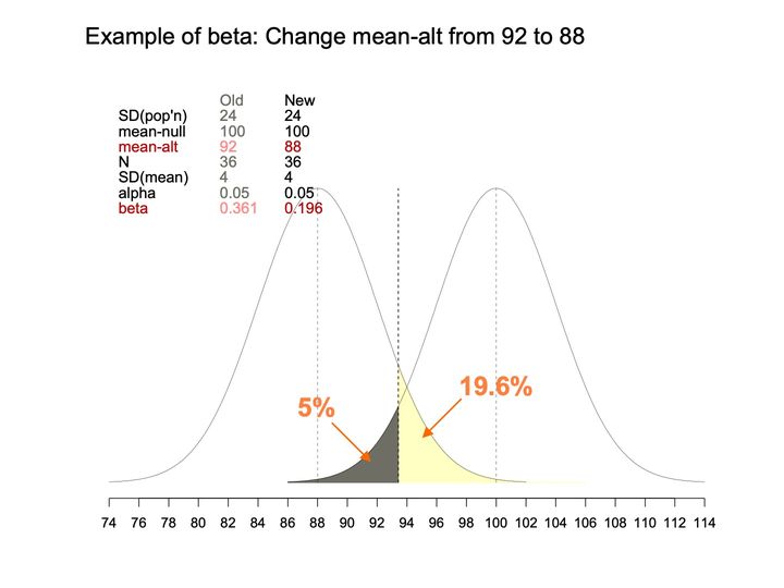
- Panels
- 1
- Elements
- 2 bell-shaped curves (thin black lines) of equal width and height, each with a thin gray dashed vertical line at its peak; 1 black dashed vertical line at a cutoff; 2 shaded areas meeting at the cutoff, one dark gray and one pale yellow; 2 orange arrows with orange percentage labels (5% and 19.6%) pointing into the shaded areas. A parameter table sits at the upper left: Old column in gray, New column in black, with the changed rows (mean-alt and beta) in red, paler red in the Old column. No legend; the curves themselves are unlabeled, and their peaks fall at the New values of mean-alt (88) and mean-null (100) in the table.
- Horizontal
- 74 to 114, labeled ticks every 2; the left curve begins near 74 and the right curve ends near 114; dashed vertical guides at about 88 and 100 (the peaks) and at about 93.4 (the cutoff)
- Vertical
- no axis or scale; both curves rise to the same height, with the parameter table filling the space above and to the left of the left curve's peak
- Visible pattern
- The 2 curves are the same shape, set 12 units apart, and overlap between roughly 86 and 102, crossing near 94. The cutoff line stands between the peaks, somewhat closer to the left one. The dark gray area is a thin sliver under the left tail of the right curve, running from about 86 up to the cutoff, where it reaches about a quarter of the peak height; the 5% label points to it. The pale yellow area lies under the right tail of the left curve, starting at the cutoff at a bit over a third of the peak height and tapering to the baseline, with a faint yellow line continuing along the baseline to about 106; the 19.6% label points to it.
Text in the picture
Example of beta: Change mean-alt from 92 to 88
Old New
SD(pop'n) 24 24
mean-null 100 100
mean-alt 92 88
N 36 36
SD(mean) 4 4
alpha 0.05 0.05
beta 0.361 0.196
5%
19.6%
Abbreviations: SD = standard deviation.
- Panels
- 1
- Elements
- 2 bell-shaped curves of the same width and height, each with a dashed vertical line at its center; a third dashed vertical line at a cutpoint; under the right-hand curve, the area left of the cutpoint is shaded dark gray, with an orange arrow from the label "5%"; under the left-hand curve, the area right of the cutpoint is shaded pale yellow, with an orange arrow from the label "36.1%"; a parameter table is placed at the upper left.
- Horizontal
- 74 to 114, ticks every 2; curves span about 78 to 114; thin dashed verticals at 92 and 100, bolder dashed vertical at about 93
- Vertical
- No axis or scale; both curves rise from a common baseline to the same peak height, with the parameter table to the left of the left curve's peak
- Visible pattern
- The 2 curves overlap broadly, one peaked at 92 and the other at 100, crossing at about 96. The bolder dashed line at about 93 divides the shading: dark gray on the left , pale yellow on the right. An arrow labeled 5% points into the gray region, and an arrow labeled 36.1% points into the yellow region.
Text in the picture
Example of beta
SD(pop'n) 24
mean-null 100
mean-alt 92
N 36
SD(mean) 4
alpha 0.05
beta 0.361
Abbreviations: SD = standard deviation.
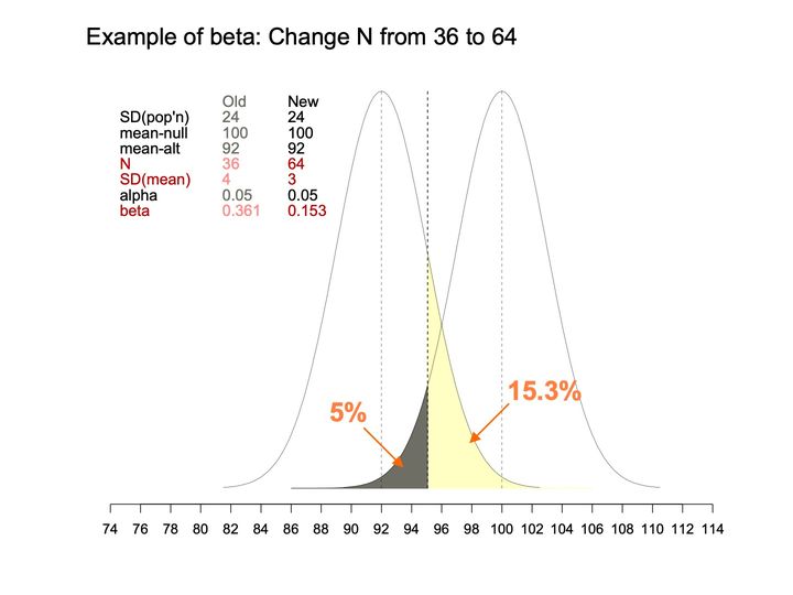
- Panels
- 1
- Elements
- 2 bell-shaped curves (thin black lines) of equal width and height, each with a thin gray dashed vertical line at its peak; 1 black dashed vertical line at a cutoff; 2 shaded areas meeting at the cutoff, one dark gray and one pale yellow; 2 orange arrows with orange percentage labels (5% and 15.3%) pointing into the shaded areas. A parameter table sits at the upper left: Old column in gray, New column in black, with the changed rows (N, SD(mean) and beta) in red, paler red in the Old column. No legend; the curves themselves are unlabeled, and their peaks fall at the values of mean-alt (92) and mean-null (100) in the table.
- Horizontal
- 74 to 114, labeled ticks every 2; the curves span about 81 to 110; dashed vertical guides at about 92 and 100 (the peaks) and at about 95 (the cutoff)
- Vertical
- no axis or scale; both curves rise to the same height, nearly to the level of the table's Old/New header, with the table to the left of the left curve
- Visible pattern
- Compared with the curves on the neighboring beta slides drawn on the same horizontal scale, these 2 are narrower and rise higher, and they overlap less, crossing near 96 at about a third of the peak height. The cutoff line stands about midway between the peaks, a little left of center. The dark gray area is a narrow sliver under the left tail of the right curve, from about 86 to the cutoff, where it reaches about a quarter of the peak height; the 5% label points to it. The pale yellow area lies under the right side of the left curve beyond the cutoff, starting at a bit under 2-thirds of the peak height and tapering to the baseline near 102, with a faint yellow line continuing along the baseline to about 106; the 15.3% label points to it.
Text in the picture
Example of beta: Change N from 36 to 64
Old New
SD(pop'n) 24 24
mean-null 100 100
mean-alt 92 92
N 36 64
SD(mean) 4 3
alpha 0.05 0.05
beta 0.361 0.153
5%
15.3%
Abbreviations: SD = standard deviation.
- Panels
- 1
- Elements
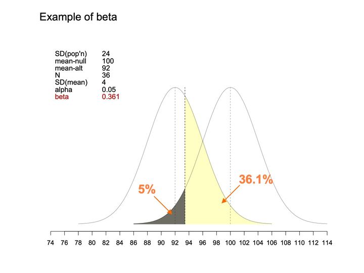
- 2 bell-shaped curves of the same width and height, each with a dashed vertical line at its center; a third dashed vertical line at a cutpoint; under the right-hand curve, the area left of the cutpoint is shaded dark gray, with an orange arrow from the label "5%"; under the left-hand curve, the area right of the cutpoint is shaded pale yellow, with an orange arrow from the label "36.1%"; a parameter table is placed at the upper left.
- Horizontal
- 74 to 114, ticks every 2; curves span about 78 to 114; thin dashed verticals at 92 and 100, bolder dashed vertical at about 93
- Vertical
- No axis or scale; both curves rise from a common baseline to the same peak height, with the parameter table to the left of the left curve's peak
- Visible pattern
- The 2 curves overlap broadly, one peaked at 92 and the other at 100, crossing at about 96. The bolder dashed line at about 93 divides the shading: dark gray on the left , pale yellow on the right. An arrow labeled 5% points into the gray region, and an arrow labeled 36.1% points into the yellow region.
Text in the picture
Example of beta
SD(pop'n) 24
mean-null 100
mean-alt 92
N 36
SD(mean) 4
alpha 0.05
beta 0.361
Abbreviations: SD = standard deviation.
- Panels
- 1
- Elements
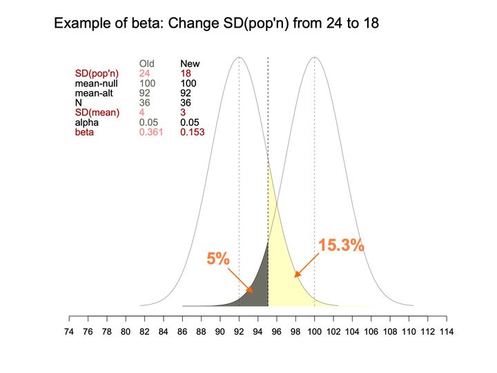
- 2 bell-shaped curves (thin black lines) of equal width and height, each with a thin gray dashed vertical line at its peak; 1 black dashed vertical line at a cutoff; 2 shaded areas meeting at the cutoff, one dark gray and one pale yellow; 2 orange arrows with orange percentage labels (5% and 15.3%) pointing into the shaded areas. A parameter table sits at the upper left: Old column in gray, New column in black, with the changed rows (SD(pop'n), SD(mean) and beta) in red, paler red in the Old column. No legend; the curves themselves are unlabeled, and their peaks fall at the values of mean-alt (92) and mean-null (100) in the table.
- Horizontal
- 74 to 114, labeled ticks every 2; the curves span about 81 to 110; dashed vertical guides at about 92 and 100 (the peaks) and at about 95 (the cutoff)
- Vertical
- no axis or scale; both curves rise to the same height, nearly to the level of the table's Old/New header, with the table to the left of the left curve
- Visible pattern
- Compared with the curves on the neighboring beta slides drawn on the same horizontal scale, these 2 are narrower and rise higher, and they overlap less, crossing near 96 at about a third of the peak height. The cutoff line stands about midway between the peaks, a little left of center. The dark gray area is a narrow sliver under the left tail of the right curve, from about 86 to the cutoff, where it reaches about a quarter of the peak height; the 5% label points to it. The pale yellow area lies under the right side of the left curve beyond the cutoff, starting at a bit under 2-thirds of the peak height and tapering to the baseline near 102, with a faint yellow line continuing along the baseline to about 106; the 15.3% label points to it.
Text in the picture
Example of beta: Change SD(pop'n) from 24 to 18
Old New
SD(pop'n) 24 18
mean-null 100 100
mean-alt 92 92
N 36 36
SD(mean) 4 3
alpha 0.05 0.05
beta 0.361 0.153
5%
15.3%
Abbreviations: SD = standard deviation.

Abbreviations: BMI = body mass index (kg/m²); HER/HERS = HIV Epidemiology Research (HER) Study; NHANES = National Health and Nutrition Examination Survey; US = United States.
Abbreviations: EIS = Epidemic Intelligence Service (CDC).


Abbreviations
BMI = body mass index (kg/m²); CDC = Centers for Disease Control and Prevention; EIS = Epidemic Intelligence Service (CDC); HER/HERS = HIV Epidemiology Research (HER) Study; HHS = Department of Health and Human Services; HIV = human immunodeficiency virus; HIV+ = HIV-positive; NHANES = National Health and Nutrition Examination Survey; ResH = research hypothesis; SD = standard deviation; SE = standard error; StaH = statistical hypothesis; SubH = substantive hypothesis; TS = test statistic; US = United States; USA = United States of America.
References, compiled for this page
Full citations, with current links, for selected references and related works.
Full references: whole site, by domain (opens in a new tab) · whole site, by type of work (opens in a new tab)
- Heilig CM. A culture for doing good things with data. 2025-04-24.On this site (opens in a new tab)
- Paramsothy P, Duerr A, Heilig CM, Cu-Uvin S, Anderson JR, Schuman P, Klein RS. Abnormal vaginal cytology in HIV-infected and at-risk women after hysterectomy. Journal of Acquired Immune Deficiency Syndromes. 2004-04; 35(5): 484–491.Elsewhere on the web (opens in a new tab)
- Phelps RM, Smith DK, Heilig CM, Gardner LI, Carpenter CCJ, Klein RS, Jamieson DJ, Vlahov D, Schuman P, Holmberg SD, HER Study Group. Cancer incidence in women with or at risk for HIV. International Journal of Cancer. 2001-12-01; 94(5): 753–757. (slide 13)Elsewhere on the web (opens in a new tab)
- Tohill BC, Heilig CM, Klein RS, Rompalo A, Cu-Uvin S, Piwoz EG, Jamieson DJ, Duerr A. Nutritional biomarkers associated with gynecological conditions among US women with or at risk of HIV infection. American Journal of Clinical Nutrition. 2007-05; 85(5): 1327–1334. (slides 7–10, 13, 72, 74, 87)Elsewhere on the web (opens in a new tab)